Introduction The page is updated regularly: Last updated: 2022-11-22 Section 19 - "XYZ-export"
The Olex machine comes with pre-installed software, and is ready for use when switched on for the first time. It must be mounted rigidly attached to the boat, preferably connected to an uninterruptable power supply (UPS).The machine is designed to always be turned on.
Installation
Unpack the machine and place it with the back side upwards on a flat surface. Screw the mounting brackets firmly onto the machine with the supplied screws.
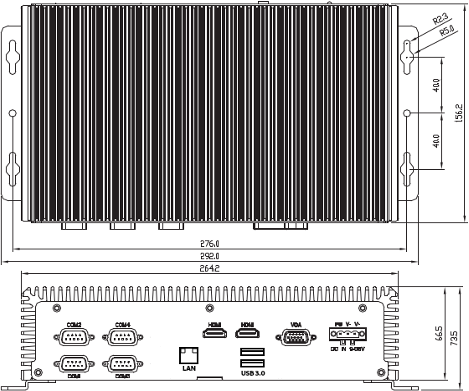
Mount the machine on a wall, or similar. Be sure that air can circulate freely between the machine and the surface.
Danger
Keep the machine away from water! Fire, electrical shock or injury can occur!!
Connect to power
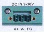
Connect the supplied green DC-connector to a power source, the machine can be operated at any voltage between 9V and 30V DC. Make sure the polarity is correct before the connector is plugged into the socket. Reversed polarity can cause fatal damage to the machine, even after a short time.
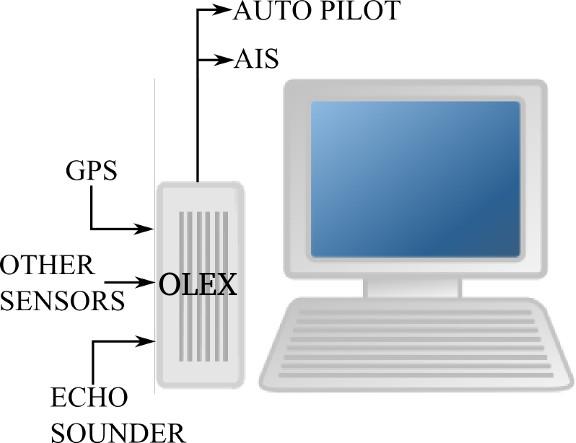
Connect monitor, keyboard, mouse and possibly other instruments such as GPS, sonar, AIS, Autopilot and radar.
Optocoupler
If there are sources of electrical noise on board, the signal at the serial (NMEA) inputs may be disturbed. An optocoupler can be connected to avoid this. An opto-isolator or optocoupler is an electronic component that transfers electrical signals between two isolated circuits using light
M4 - front side
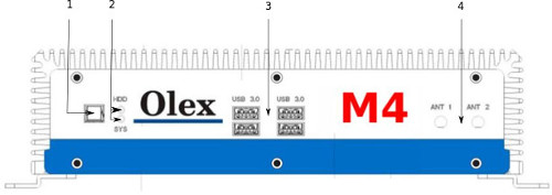
- Power-switch
- System indicator and Harddrive indicator
- USB ports
- WIFI-antennas
M4 - back side

Display settings and screen resolution
Olex may be connected to one or more monitors, either via VGA, DVI, HDMI or USB. Number of connected monitors is ulimited. It is easy to choose screen resolution, define right and left display - or whether both (all) monitors should display the same image. Click Layers → Display settings to open the Display panel - all available monitors are listed here. The panel views the monitor name, connection method and format (widescreen/normal). In addition the screen resolution for each monitor is listed, and whether the monitor is defined as left or right.
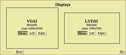
- Mono - Single display image, copied to all connected monitors.
- Left - Dual display left image - navigation image with all menus and information bars.
- Right - Dual display right image - full screen 3D view, overwiew map or available echograms.
One monitor
Choose between available screen resolutions by clicking Previous or Next, and then Set to select. Answer "Yes " when "Do you really want to change the display settings? " opens. And confirm when "Can you see the image? " appears. If the screen image is out of range, click "No " or wait until the red bar disappers. Select another screen resolution and try again. Click "Ok " to close the panel.
Two or more monitors
With several monitors connected, the options are, either to define Left/Right image for dual display, or select Mono for single display on all monitors. A red frame will appear both in the middle of the Display panel and outline the selected screen, when the mouse cursor is moved inside the Display panel to view which monitor is to be changed.
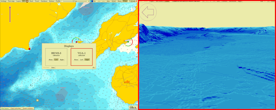
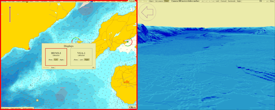
To choose display method, click Left, Right or Mono. Common screen resolutions for all monitors are listed in the lower left part of the Display panel. To change resolution, click Previous or Next, and select resolution by clicking "Set ". Confirm with " Yes ". If the image looks nice, answer the question " Can you see the image? " with "Yes ". If not, click "No " or wait for the time out. Select another screen resolution and try again. A click on "Ok " in the lower right corner, closes the panel.
Widescreen and standard monitor
The display settings will show suitable screen resolutions common to all the connected monitors. If a widescreen and a standard monitor are connected at the same time, any common resolutions might be limited. Similar monitors are therefore recommended.
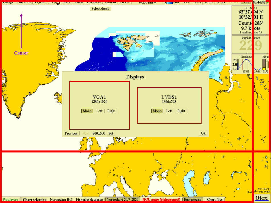
The red frames previews the screen sections to be displayed on the widescreen and the standard monitor respectively.
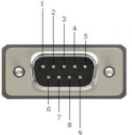
Serial port pinning
| PIN | SIGNAL | I/O |
|---|---|---|
| 1 | DCD - Data Carrier Detect | I |
| 2 | RxD - Receive Data (data from computer to instrument) | I |
| 3 | TxD - Transmit Data (data from computer to instrument) | O |
| 4 | Data Terminal Ready | O |
| 5 | Common 0V | |
| 6 | DSR - Data Set Ready | I |
| 7 | RTS - Request to send | O |
| 8 | CTS - Clear To Send | I/td> |
| 9 | +5V - Ring indicator | I |
Starting Olex
Start the computer by pressing the "power-button" once. Before the system is ready, it will go through a start-up sequence where different screens occurs in order as the sequence is completed.
Warning
Do not turn off the machine during start-up, as this may damage the Olex installation!
After a few seconds the machine will halt, and a blue screen with an overview of available screen configurations is displayed.
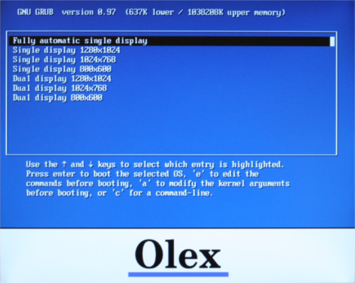
On initial startup or when changing monitor, select screen configuration by using the arrow keys to move the marker up or down. The recent screen settings will be highlighted next time the system is started.
Press Enter to proceed or wait until the machine boots automatically. The machine halts again when the window displaying the software rights opens
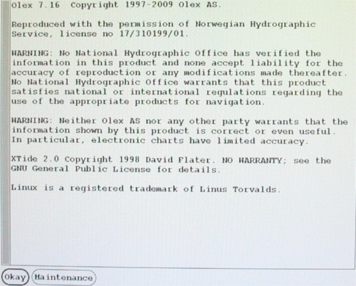
Click Okay to confirm, or wait until the start-up procedure resumes automatically. Click Maintenance to open maintenance mode.
Upgrade Olex version
Find and download the latest Olex-version at www.olex.no
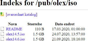
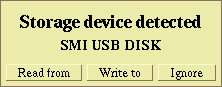
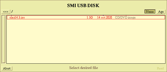
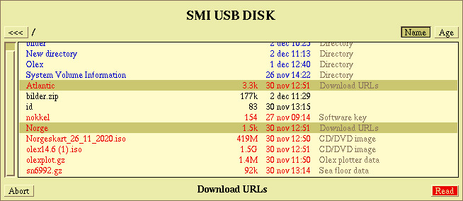
Click on one of the .iso files, and save it to a USB memory-stick. Connect the device to the Olex machine and click Read from.
When the filebrowser opens, click on the.iso file.
and then click inside the filebrowser window to select all the files.
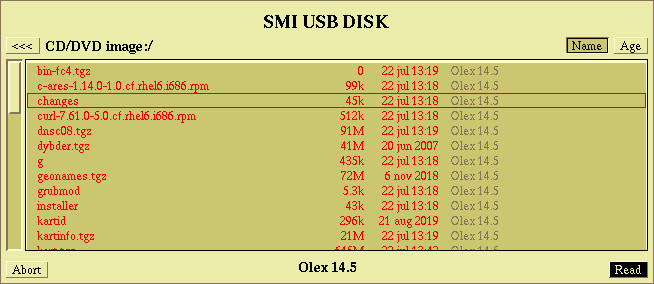
Click Read, and confirm when asked "Olex 14.5 - do you really want to read?" A window showing the innstallation progress opens, any possible error messages will be displayed in this window.
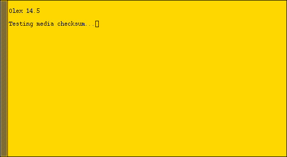
The computer restarts when the installation is complete.
WI-FI
In order to download weather files and other types of data, the machine must be connected to a network. M4 is the first Olex machine with built-in WiFi. However, most older machines can be connected to WiFI using a WiFi dongle connected to one of the USB ports. The Internet icon in the upper right corner indicates whether the machine is connected to a network.
 = no network connection
 = connection OK
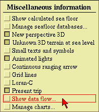
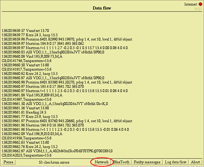
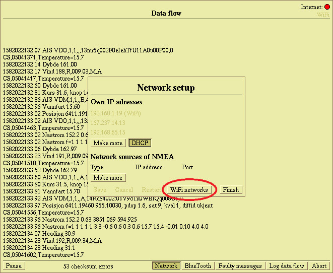
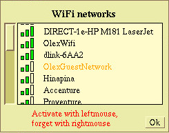
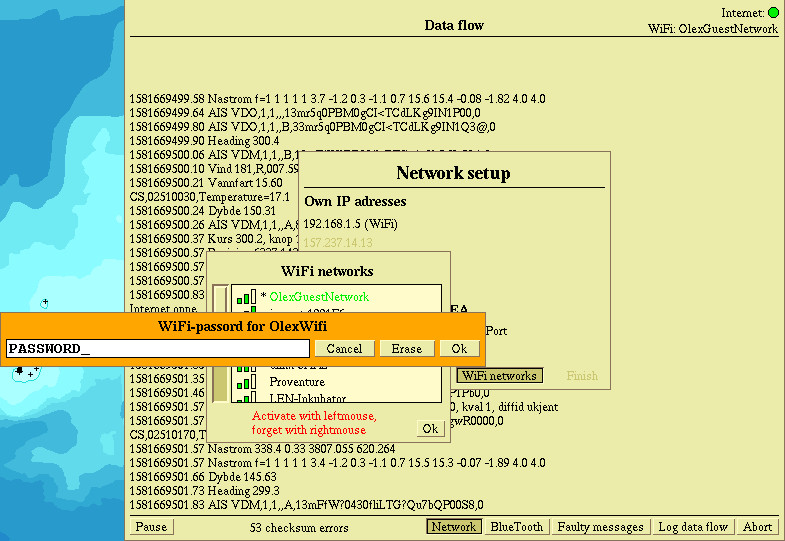
Click Layers → Show data flow → Network → WiFi-networks to open a window with a list of available WiFi networks. Note that the WiFi Network button is available only on machines with hardware for wireless network connection.
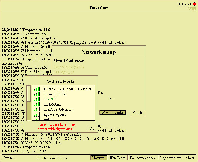
The network names are listed in order of signal strength. Networks where the name is marked with an asterisk already have a saved password, and there is no need to re-enter when connecting to the network.
Connect with WiFi for the first time
Use the left mouse button to select a network, then enter the WiFi password in the box that opens.
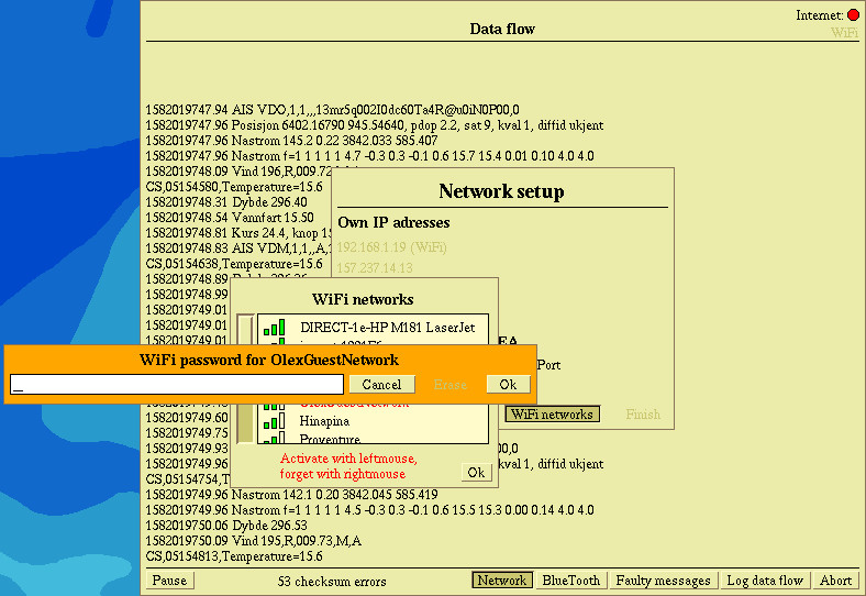
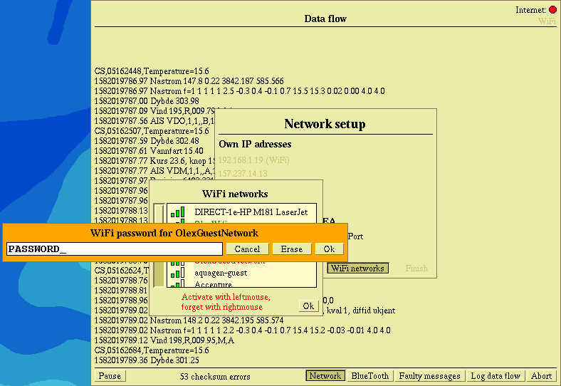
Click Ok to confirm and connect, or click Cancel to cancel and close. Erase deletes the charachters in the password field. While the machine is connecting to the network and verifiing the password, the network name will temporarly become orange and the network indicator will be red.
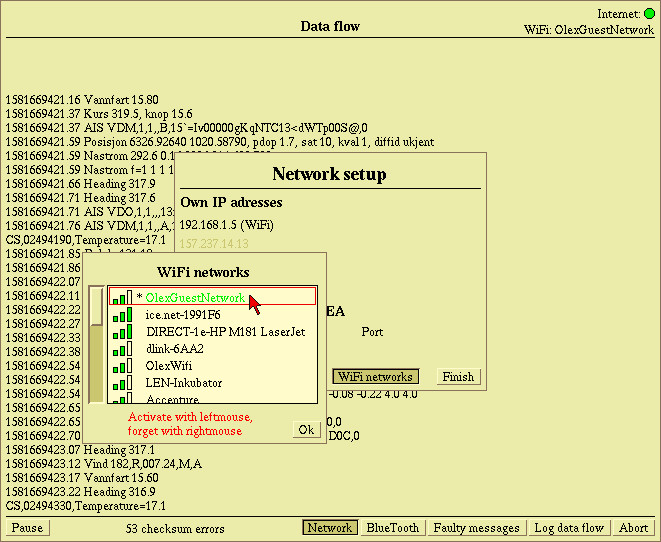
When the connection is established, the network name and the indicator in the upper right corner will turn green. And the network name will appear in the upper right corner of the �Data Flow� window. It may sometimes take a few seconds for the network to be ready for use. Click Ok → Finish → Abort to close the �Data flow�-window.
Switch between networks
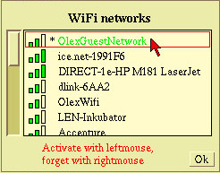
Click Layers → Show data flow → Network → WiFi Network to open the �WiFi Networks� window, and select network by left-clicking on the network name. If the network has been connected before and the password is saved, the name will be marked with an asterisk and there is no need to re-enter the password. Recent connected networks will appear with dark green font in the list.
Delete a network
To delete a network, go to the �WiFi network� window and right-click on the network name. Confirm by clicking "Yes". Then the network password is deleted and must be entered again if this network is to be reconnected.
Enable the firewall in Olex
When connecting the machine to the internet, it is recommended to enable the firewall. If the machine is turned off, select Maintenance at startup. If the machine is already on, press Ctrl + Shift + right mouse button and the Maintenance window opens.
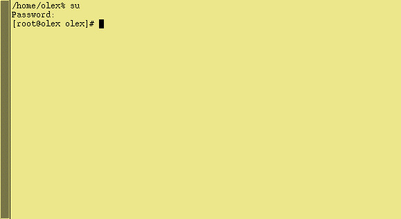
Point the mouse pointer inside the window. Change the command prompt to "root" by typing "su". Enter "fishbat" when questions about password appear. Press OK to confirm
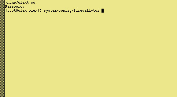
Open the firewall user interface by entering:"System-config-firewall-tui".
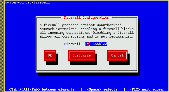
Use the spacebar to enable Firewall
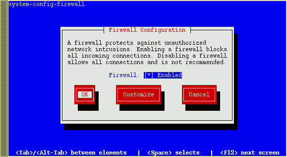
The use the Tab key to go to "OK". Press Enter to cinfirm.
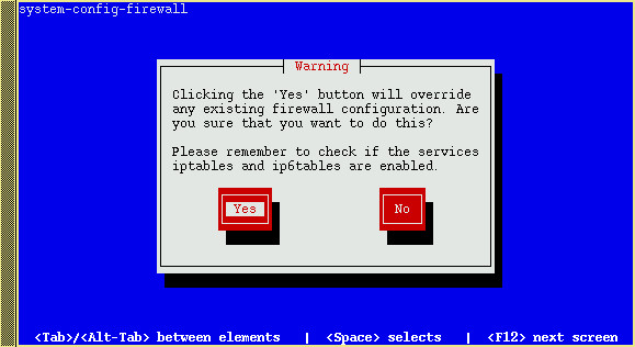
Select Yes and finanlly Enter to exit.
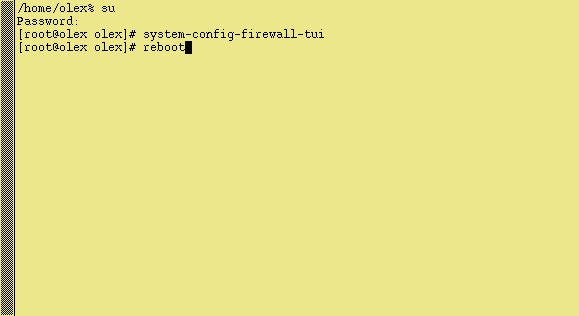
Enter "reboot" and then press Enter to restart the machine.
Connect the network cable to the machine. To test if the machine is connected to the network, open the data traffic window. Click Layers → Show Data flow.., in the top right corner, the indicator for the internet will light green. If indicator is red, this means the machine is not in contact with the internet. If so, check the internet connection again.
Basic operation
Olex is a complete system for seabed mapping, plotting and navigation. By using GPS and echo sounder - position- and depth data are measured and saved to the system. These data are continuously recalculated and added to previous measurements. The result is visualized as a realistic 3-D image (3D-map) of the seabed. The system have advanced features for navigation, with possibility of software extensions for e.g. weather, multibeamsounders, trawl/ROV positioning, AIS and oceanic currents measurements.
The most widely used installation is on the M4-machine, but Olex can also be installed on a laptop or desktop PC. Olex can be operated both with a mouse and keyboard. The keyboard is used for entering names and comments, and also for using hot keys. The mouse is used for zooming in and out, grab objects and select options in the menus.
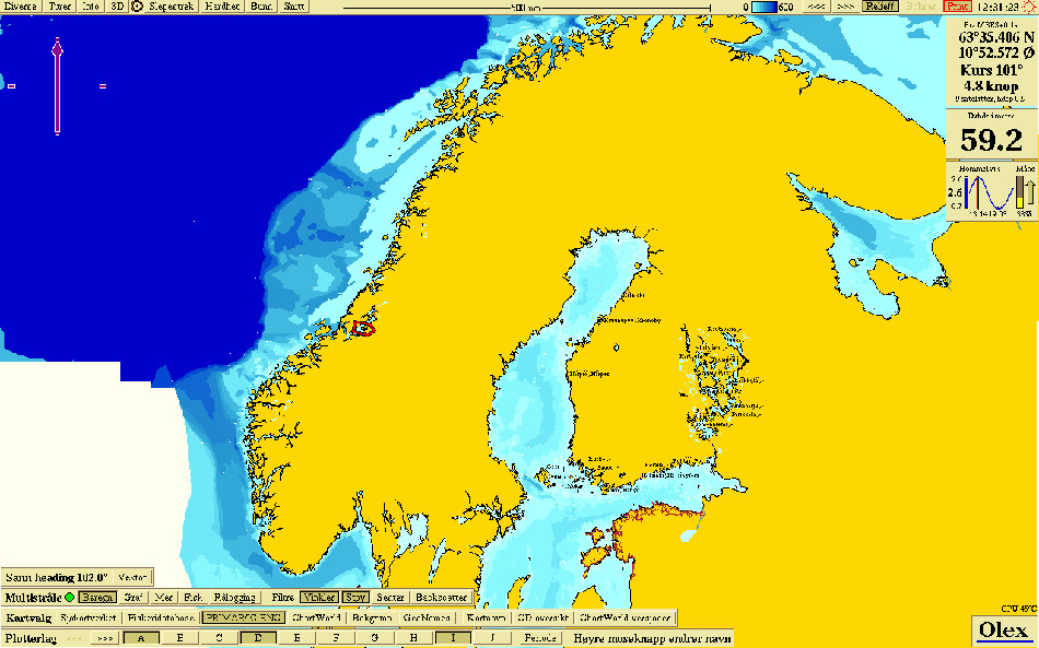
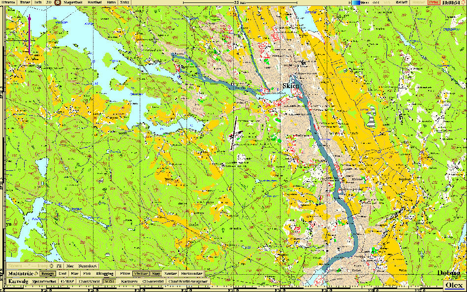
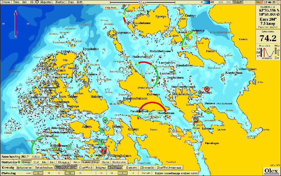
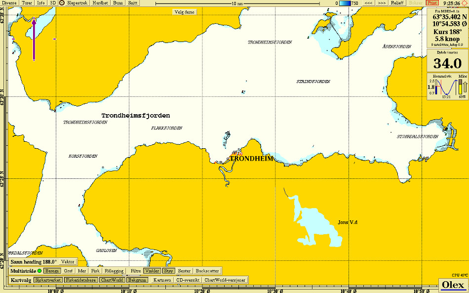
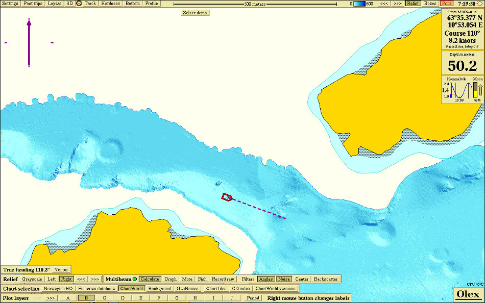
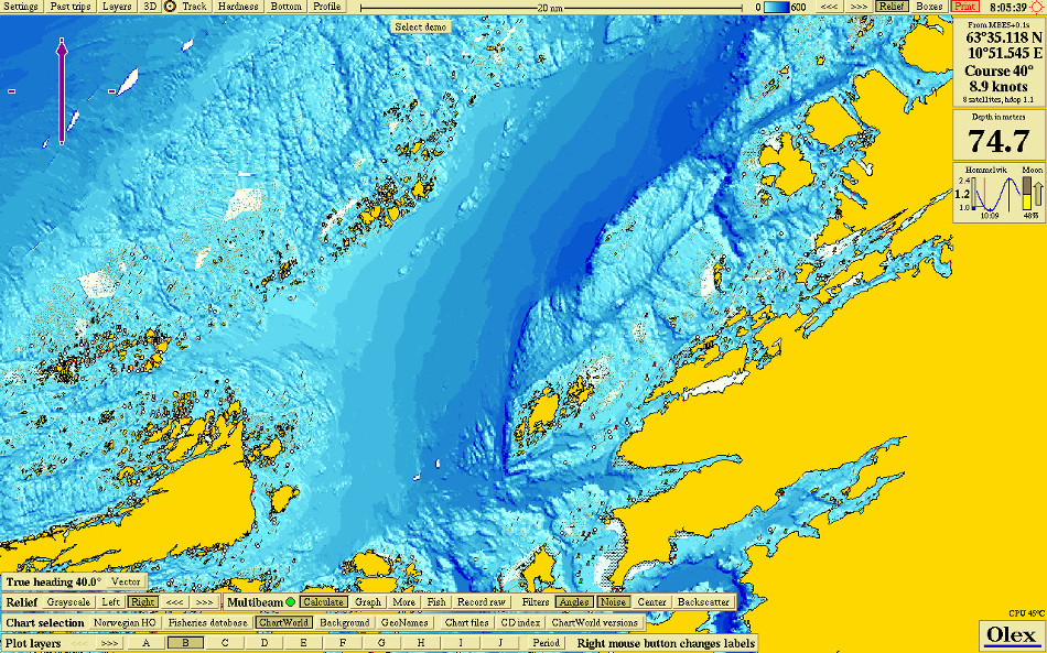
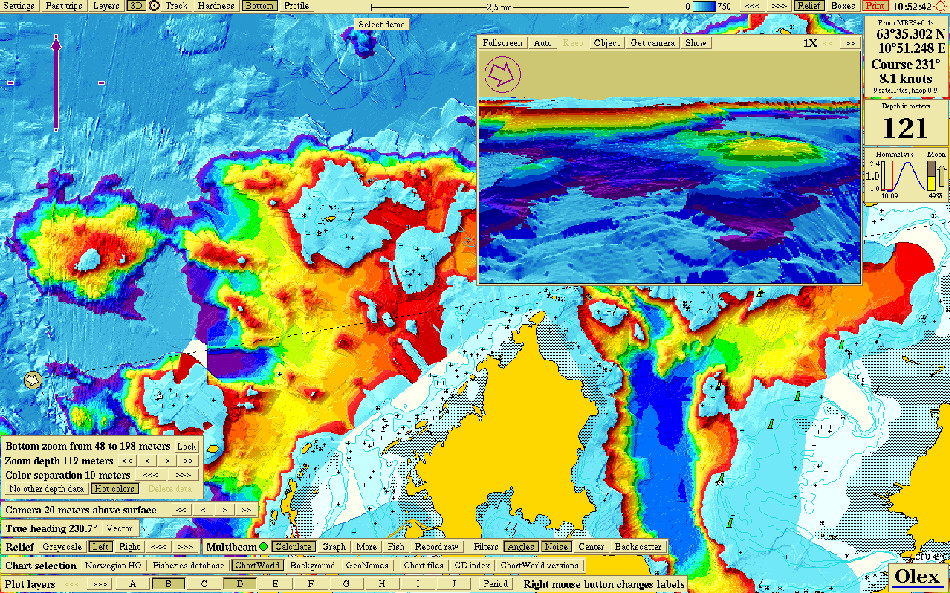
The main screen
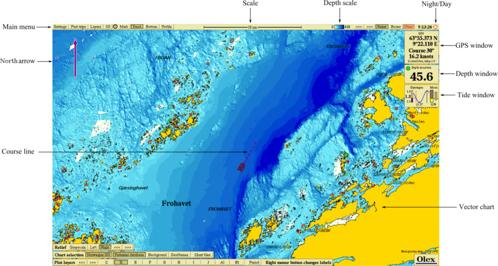
Typical view with the ship sailing towards northeast in the middle of the screen.

Symbols and objects
Some objects will change color or appearance when the mousecursor is moved around and touches them. The map is zoomed in by clicking the right mouse button, left mouse button zooms out. There are also other ways to zoom in and out. When the map is zoomed in to a certain scale (100 metres), a marker showing the depth value in that point is opened, if measured depth values excists in that point.

The main menu at the top of the screen has several drop-down menus, and buttons that provide access to various functions. Like changing the chart scale, adjusting colors and night dimming. The GPS window is located in the upper right corner, and provides information about the position, course and speed.
The depth window displays the depth value of the last sounding. By clicking inside the panel, a more detailed view is opened.
The tide window displays the nearest station for tidal measurements, the present water level, and the time for the next high and low tide.
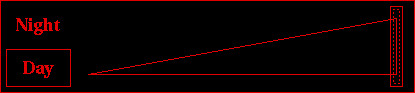
The brightness can be adjusted by using the dimmer function. The dimmer panel appears when the mouse pointer touches the sun icon in the upper right corner

The brightness can also be adjusted by moving the slider along the scale. Switch between day- and night colours by clicking Day or Night.
North-arrow
Touch the arrow in the upper right corner. A panel ,where to change the ship's location on the screen and orientation of the map, opens.
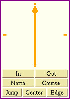
Grab the north-arrow to rotate the map in any direction, the arrow always always points towards north.
- In - zooms in.
- Out - zooms out.
- North and Course - changes the map's orientation.
- Jump - the ship moves across the screen, while the map is stationary.
- Center - the ship is always located in the center of the screen. If the chart is moved when Center is activated, by using the arrow keys or the mouse, the text below the arrow will change to "New Center".
- Edge - the ship is always located near the edge of the screen, with most of the chart area in front of the bow.
Zooming and rotation leads to a temporary change of view, and the buttons Keep this and Go back opens in the upper part of the screen.
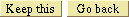
By clicking Keep this, the new setting will be retained. Go back resets the screen immediately. After a period of inactivity, the screen settings will automatically be reset.
Zooming
The map can be zoomed in and out in different ways to see details.
- Use the left mouse button to zoom in, and the right mouse button to zoom out.
- Use the buttons In or Out beneath the north-arrow.
- Move the mouse scrollwheel forwards to zoom out, or backwards to zoom in.
- Click on the chart scale in the main menu, left-click zooms in, right-click zooms out.
- The Page Up and Page Down keys zoom in and out respectively.
Moving the map
The map can be moved in any direction:
- Press the scrollwheel or the middle button on a 3-button mouse. Move the mouse while the button is pressed.
- On a 2-button mouse, hold down both buttons simultaneously.
- Use the arrow keys on the keyboard to move the map.
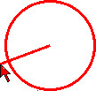
- Press and hold the middle mouse button or the scrollwheel. Then press and hold one of the other buttons as well. A red circle appears. Move the mouse away from the circle and the map will continuously move in the opposite direction. By moving the mouse pointer, the map will move in steps in the opposite direction, proportional to the lenght of the red line. When the line is short map will move slowly, and when the line is long the map will move faster.
Buttons and panels
Some buttons opens new menus, and others activates functions.
 - The button is not activated
 - When the button is touched, both the text and the frame will turn red.
 - The button is activated.
 - If the function is unavailable, the text is light gray,
and it is not possible to click on it.
- If the function is unavailable, the text is light gray,
and it is not possible to click on it.
 - Some buttons have a little gray check box to the left of the text.
The function is activated by clicking somewhere inside the red frame.
- Some buttons have a little gray check box to the left of the text.
The function is activated by clicking somewhere inside the red frame.
General navigation
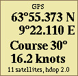
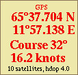
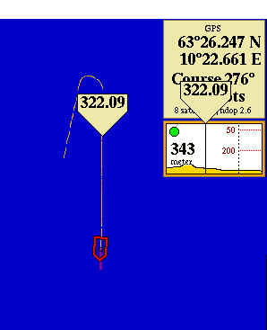
Position from GPS
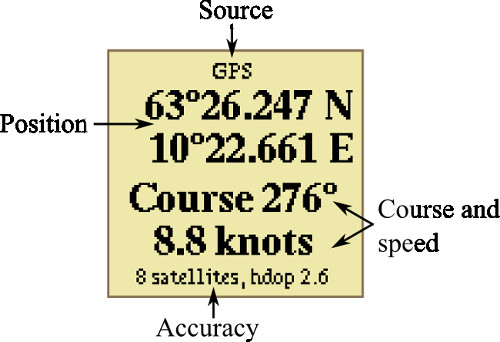
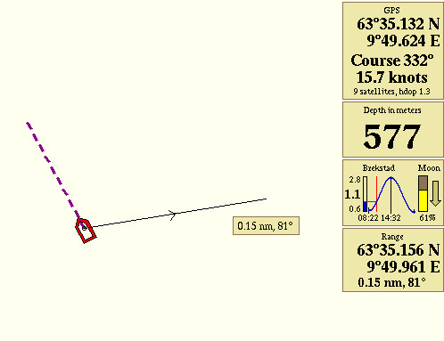
Position, course and speed is displayed in the GPS panel. These data are usually provided by the GPS receiver, but can also come from other sources such as AIS, radar or a multi-beam echo sounder. If multiple sources are available, signals from the GPS receiver are given priority. If positioning messages from the GPS is not available, the system will use messages in order of priority from the AIS, multi-beam echo sounder or radar.
Change view by clicking repeatedly inside the window.
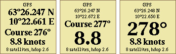
The bottom line shows the number of satellites and quality of the position. Low HDOP - horizontal dilution of precision, means good position accuracy. Numbers below 4 are considered as good positioning accuracy. If the quality of the GSP signal is poor, the numbers will turn red and the seabed calcultion will halt.
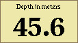
Depths from echo sounder
The depth panel displays the depth of the last sounding. The depth values may be provided by a single beam echo sounder, or a multibeam echo sounder. If there are more then 30 seconds from the last received depth message, the numbers will turn gray. This time may vary, depending on the type of echo sounder.
If Settings → Show calculation progress is turned on, a green dot flashes in the panel for each registered depth echo. If the echo sounder detects hardness, this dot may appear in different colours.
 - both depth and hardness are registrated
 - depth values are registrated, no hardness
 - no depts nor hardness values are registrated
By clicking inside the depth panel, an echogram displaing the last measured depths opens.
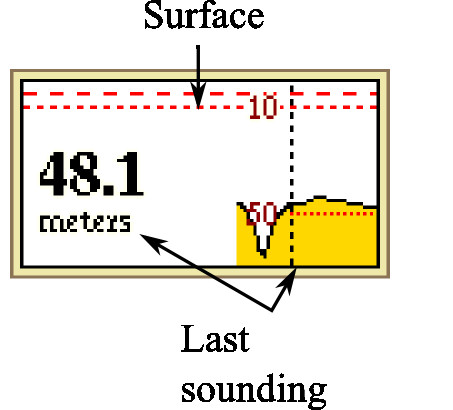
When the cursor is moved inside the echogram window, a flag displaying the depth value is opened. The depth value is also shown at the corresponding location on the map.
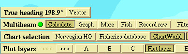
Heading
The heading shows the ship�s orientation - the direction the bow is pointing towards. The heading data may be provided by a GPS compass, magnetic compass, radar or an other heading source. If several heading sources are avilable, true heading from GPS is given priority. True heading - orientation relative to geographic north. Magnetic heading - rientation relative to the magnetic north pole. The heading is specified in degrees, and appears as a solid line along the ship's center line.
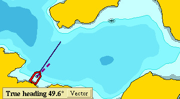
By clicking Vector the heading line is extended.
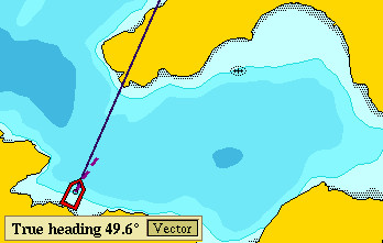
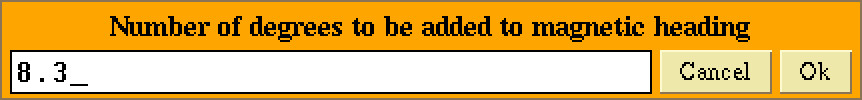
If the heading signal comes from a magnetic compass, "Magnetic heading" will appear , in stead of "True heading" in the panel in the bottom left corner. By clicking Adjust a new window opens in which it is possible to write corrections for the deviation between true heading and magnetic heading.
Roll and pitch
When the machine receives data about the ship�s roll and pitch, these data can be displayed by clicking Settings → View roll and pitch.
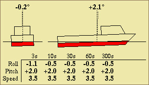
The numbers by the boat symbol displays the current values, while the table displays average values over some time.
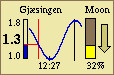
Tides
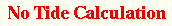
Depth values from the echo sounder are corrected for the tide level. This function is turned on or off by clicking Settings → Adjust bottom calculation for tide level. This function should always be turned on, except while doing surveys in lakes and rivers. When the function is turned off, the warning "No tide calculation" is displayed.
The tidal window displays the name of the tidal station, moon phase and time for the next high or low wather.
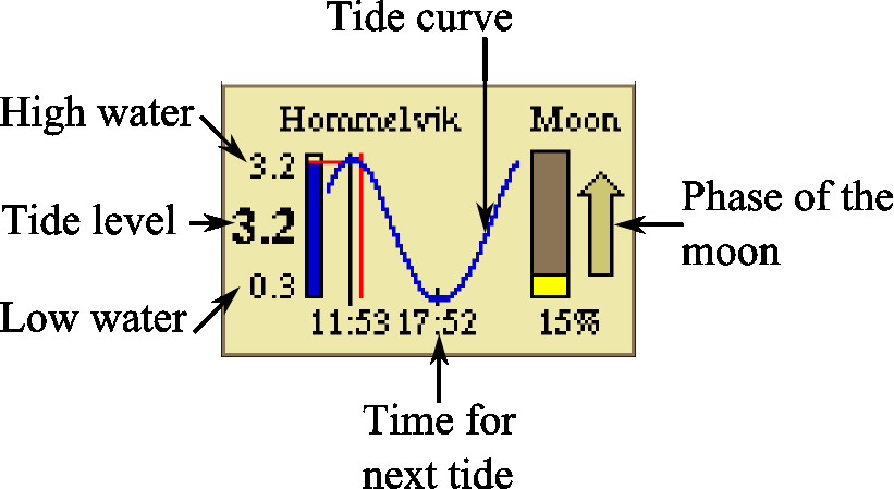
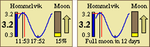
The column to the left displays the tidal level, the red cursor displays the current water level and time in the tidal cycle. The time beneath the curve indicates the time for the next high or low tide. The arrow to the right displays the moon phase. When the tide panel is touched with the cursor, the time until the next full moon is displayed.
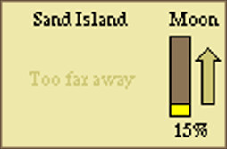
Tidal corrections are based on measurements from the Norwegian Mapping Authority over the past 30 years. Olex chooses the nearest tide station atomatically. If the distance to the nearest tide station is more than 100 nm, the tidal calculation will stop and the panel disappears from the screen.
Continuously updated ship position
The ship symbol usually moves across the screen in steps, based on the frequence of when the GPS receives positioning signals. For high-speed vessels, the function Settings → Continuously updated ship position should be enabled. The ship symbol�s location will be updated continuously based on the current speed and course.
Continuous ranging arrow
To find the distance and heading between the ship and a given point / object, the function Continuous ranging arrow can be used. Click Settings → Continuous ranging arrow. A line with starting point at the ship, and end point in the cursor will appear on the screen. The corresponding information panel with positioning information, length and direction will open on the right side beneath the Tidal Panel.
Plotter data
Plotter objects
Plotter data, or plotterobjects are marks, line objects and areas, visualized with different types of symbols in the map.
This data are organized in plot layers, and saved in a specified file on the computers harddrive. There are no limits to the amount of data that can be stored.
Mark
A mark can be one single object, or several marks can be connected to form lineobjects. Marks can be displayed with different symbols, a name and text comments. Choose a mark by clicking it once. A mark can be edited by doubleclicking it, or by first choosing the mark and then click Edit.
 - not chosen.
 - chosen mark.
 - the mark is chosen and editable.
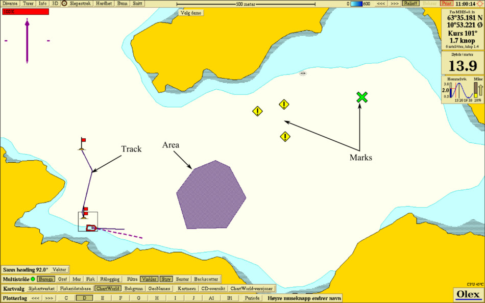
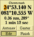
Chosen-mark-panel
When a new mark is placed, or an existing mark is chosen - the Chosen-mark-panel opens.
This panel displays the position, and also have 4 buttons. Autonav, Report in!, Edit and Finish.
- Autonav - is used for navigation towards the mark.
- Report in! - is used for reporting fishing gear to the government.
- Edit - opens the Edit-panel.
- Finish - closes the panel, and saves the settings.
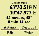
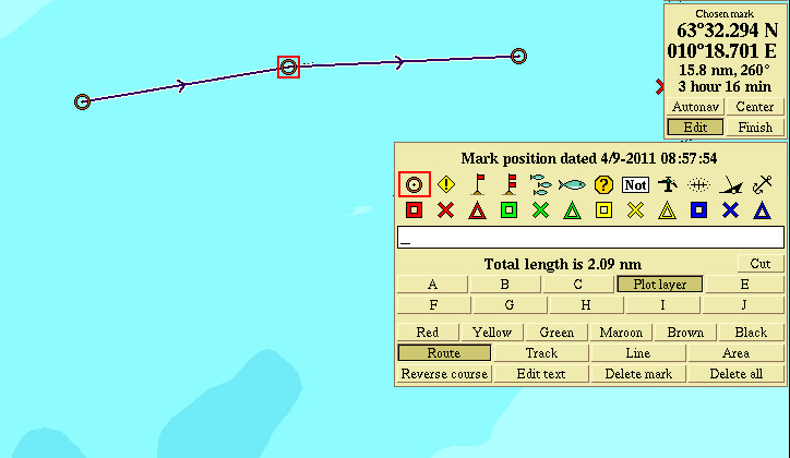
Edit-panel
This panel opens when a plotter object is created or edited.
- displays the timestamp when the mark is created or changed.
- displays the symbols to choose between.
- the mark can be named by writing in this text box.
- Plot layer assignment can be set by selecting one or more of the plotlayers.
- Edit text makes it possible to add a text comment.
- Delete mark removes the mark.
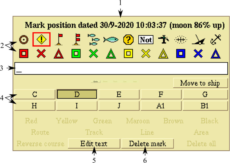
Create a new mark
Zoom in until the appropriate screen section is displayed. Grab the mark symbol in the main menu, and drag and drop the mark on the selected location.
Or hold the �Alt-button� and left-click to place a mark. Once the mark is placed, both the Chosen-mark-panel and the Edit-panel opens.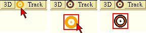
Choose a symbol in the Edit-panel, otherwise the standard symbol will be used.
- Name the mark, by entering text in the text-field.
- Determine the plot layer assignment. If not, the predefined plot layer assignment is used.
- By clicking the Edit text button, a large text area opens. Additional text comments can be entered here. Click Edit text once more to close the text editor. Click on the square on the line object to open and close the text comment.
- Click Finish to save the changes.
Edit a mark
To edit an existing mark, first open the mark for editing and make the changes. Click Finish to close and save the mark.
Placing a mark on a given position
- Place a mark at any position.
- Place the mouse cursor over the first number in the Chosen-mark-panel. Enter a value,
or click with the right or left mouse button to change the value.
Delete a mark
First open the mark for editing, and then click Delete mar. The mark with name and any text comments will be deleted.
Event mark
An event mark is placed on the ships position �right now�, and can be created by pressing any key on the keybord. The symbol can be changed by clicking Layers → Default settings for new data.
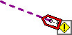
This mark can edited in the same way as any other marks.
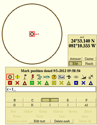
Circle with a given radius
- Place a mark at a selected position. Enter r = the value in nm in the textarea in the Edit-panel.
- A circle with the entered radius is drawn with the mark in center.
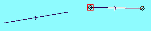
Line objects
Line objects are lines, tracks, routes and areas. There are only minor differences between this objects, and they are generally handled he same way. A line object consists of 2 or more marks connected with straight lines.
Chosen-line panel
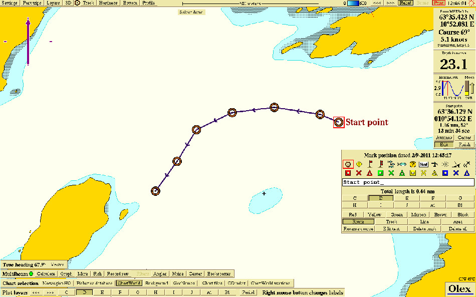
When a line object is placed, the Chosen-line-panel opens.The text �Chosen line�, �Chosen track� or �Chosen route� appears in the upper part of the panel depending of type of line object. In addition, there will be the length of the lineobject, date and name of start- and stop mark. If the line object is an area, the length will be the length of the line delimiting the area.
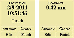
The panel have 4 buttons, Autonav, Center, Edit and Finish.
- Autonav - starts navigation towards a selected mark on the line object.
- Center - centers the line object on the screen.
- Edit - opens the Edit-panel for editing settings.
- Finish - closes the panel, and saves the settings.
Edit-panel for line objects
This panel opens when a line object is created or chosen. In top of the panel the timestamp, when the line object is created or changed, is displayed.
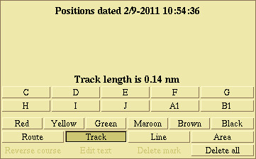
The panel has buttons for layer assignment, choice of color and for chosing the type of line object. In the lower left corner there is a button named Reverse course, this changes the direction of the line object.
By clicking Delete all, the line object with all marks will be deleted.
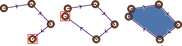
Create a new line object
- Place a mark somwhere on the map. The Chosen-mark-panel and the Edit-panel will open.
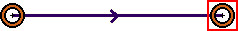
- While the mark is editable, place a new mark. The marks will be connected with a straight line, and an arrow shows the direction of the line.
- Add more marks at the end of the line, or create new marks by clicking somewhere on the line between the marks.
- Choose the type of line object by clicking one of the buttons Route, Track, Line or Area.
- Choose the color by clicking on one of the colors.
- Choose plot layer assignment by clicking on one of the plot layer buttons.
- The line can be given a name by entering text in the text field.
- Save the line object by clicking Finish.
Modify an existing line object
- Choose the line by clicking on it, the line will start flashing and the Chosen-line-panel will open.
- Click Edit, and the line object can now be edited.
- When finsihed editingm click Finish to close the panel and save the changes.
Placing a linje object on a given position
- Place a mark, and enter the position.
- Enter a comma (,), and type the position of the next turning point. Continue until the line object is completed, and click Finish in the Chosen-line-panel to save and exit.
Delete a line object
- Choose the line object by clicking it, and choose Edit from the Chosen-line-panel.
- Click Delete all in the Edit-panel. The line and all marks, names and text comments will be deleted.
Line
A line is the simplest of the line objects. A single line object consistes of two marks connected with a straight line. A line can be very complex, consisting of several hundreds of marks.
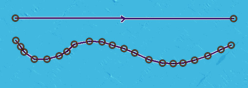
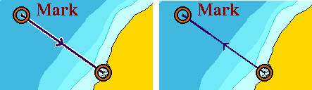
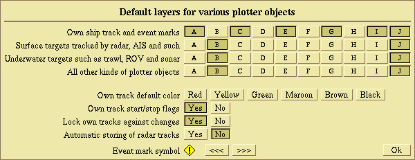
Track
A track is a line object that is recorded in the wessels wake. Click Track to start recording. A start flag is placed in the start of the track, and a solid line is recorded along the course. Click Track once more to stop recording the track line. A double flag is placed on the end mark.
Click Layers → Default settings for new data to change the color. Own track start- and stop flags, lock own tracks against changes and automatic storing of radar tracks can be changed here by clicking Yes or No on the corresponding choice. Click Ok to save the changes and close the panel.
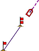
Route
A route is a track with direction towards a spesific point.
Create a route from trip
A trip can be converted to a route. Find the trip, and click Rescale according to this trip in the Past trips menu. Then click Make route from trip.
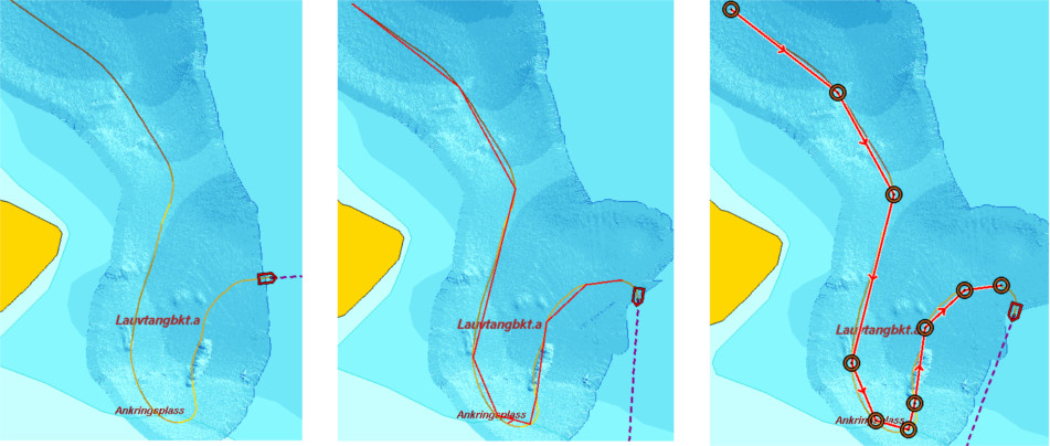
A new line object is drawn along the trip. Choose the route by clicking it, the marks will be visible and the Chosen-route-panel opens. Click Edit, and then click Unlock in the Edit-panel. Confirm when asked �Do you really want to turn off the protection?� Click Finish to save and close the panel.
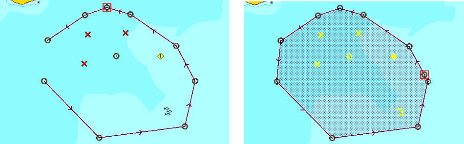
Area
An area is a line object where the first and last mark are connected.
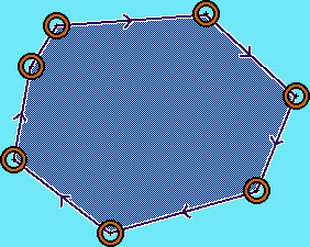
Create a new area
- Start by creating a new line object as described in earlier.
- When all the marks are placed, click Area in the Edit-panel. The first and the last mark will now be connected, and the area delimited by the lines will be filled with a color. The pattern color can be changed by clicking on one of the color options in the panel.
- Click Finish, and the area is created.
Select the area by clicking on the line object. When the area is chosen and editible, it is possible to move the line segments, add or remove marks, change color and so on.
Plot layers
Olex has 60 plot layers named from A to J5. Single plot layers can be turned on or off, by clicking on the buttons in the bottom row of the screen. A plotter object is visible when it�s corresponding layer is turned on.

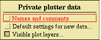
Click Layers → Visible plot layers to turn the row of buttons on or off. Left <<< and right >>> arrows are used to scroll back and forth through the plot layers. Period displays the plotterdata sorted chronologically. Click on the arrows to the right to select the timespan. Plotter data stored during this period will be displayed on the screen. When a plotter object is created, the plot layers assignment can be set manually. Otherwise the object will be automatically assigned to a preset layer.
The objects are preassigned to different plotlayers.
| LAYER | OBJECT TYPE |
|---|---|
| A | Own ship track and event marks |
| B | Surface targets tracked by radar, AIS and such |
| C | Underwater targets such as trawl, ROV and sonar |
| D | All other types of plotter objects |
This settings can be changed by opening the panel named Default layers for various plotter objects. Click Layers → Default settings for varoius plotter objects to open.
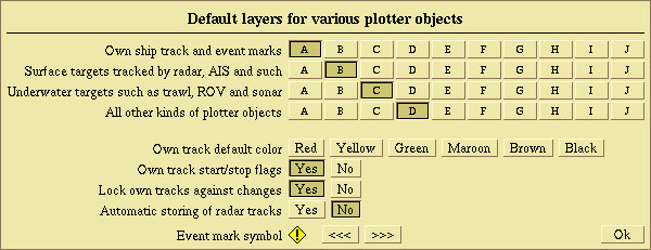
The 4 top rows of buttons defines the assignment for the plotterobjects. It is possible to select several plot layers for each object, but all objects have to be assigned to at least one plot layer. For this reason it is not possible to deselect a plot layer before selecting at least one of the other layers.
When finished editing, save any changes ond close the panel by clicking Ok
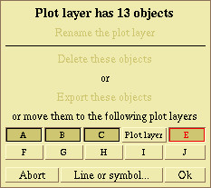
The plot layer panel
When an object is touched by the mouse cursor, the text and frame on the corresponding plot layer button will turn red.
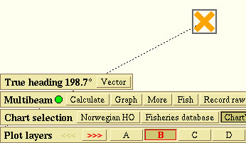
Open the plot layer panel by right clicking one of the plotlayer buttons.

This panel makes it possible to change layer assignment, plot layer name, and export data.
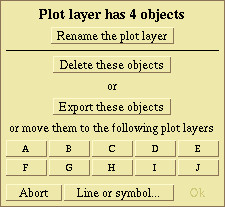
All objects assigned to this layer starts flashing when the panel is opened.
Rename the plot layer
The plotlayers are named with letters from A to J5, but can easily be renamed. Click Rename the plot layer, enter the new name in the textbox and click Ok.
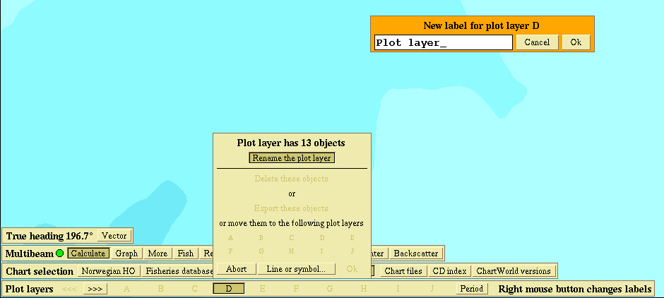
The new name now appears on the plot layer button.
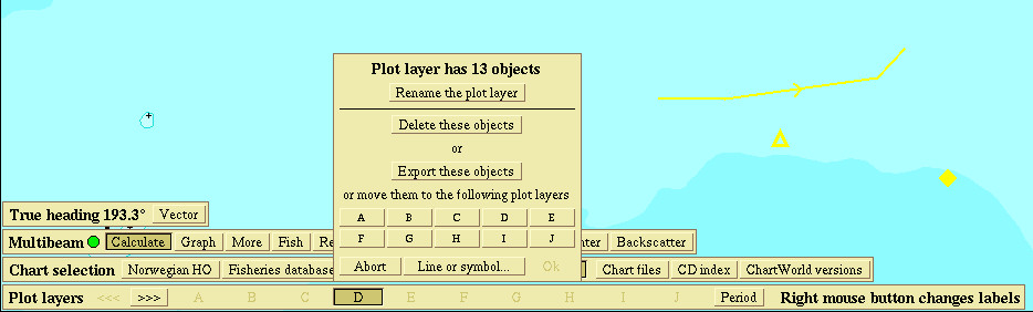
Delete plotter objects
Delete all objects assigned to a layer by clicking Delete these objects. Confirm when asked � Do you really want to delete all these plotter objects?�. It is possible to sort plotter objects, and delete only a selection.
Export plotter data
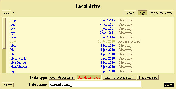
Plotterdata can be saved to local disc or to an USB device. Click Export these objects, and select a location for saving the file
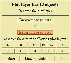
Type a new file name, or use �olexplot.gz� as the system itself suggests. Click Save, and confirm when asked � Selected plotter data - do you really want to save?� It is possible to sort plotter objects, and save only a selection.
Reassign plotlayers
The plot layer assignment can be changed by clicking on the buttons in the panel.
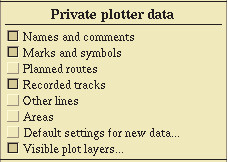
Plotterdata from old Olex versions
In previous Olex versions, the plotter data were divided into marks, routes, tracks, lines and areas. This objects was displayed by clicking the corresponding button for each object, in the Layers menu. If the computer contains old format plotterdata, the Layers menu will have checkboxes for using this data.
Save own plotter data
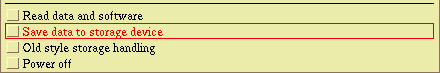
To save own plotter data, open the file browser either by choosing Settings → Save data to storage device. Select the device to store the data, and click All plotter data.
Sorting objects
Plotter objects can be sorted, to delete or export a selection of objects.
Sorting objects by the use of an area
Create an area that includes the objects to be deleted or exported. Click Objects in the Edit Panel and the objects inside the area will begin to flash yellow.
Grouping identic objects
Objects with identic symbols that belongs to the same plot layer can be grouped by clicking Line or Symbol at the bottom of the Plot layer panel. A new line opens, choose symbol by clicking on the arrow to the right or left. When the symbol is displayed in the panel, all identic symbols are displayed in yellow on the map.
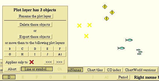
The objects can be exported, deleted or regrouped to other teams.
Split and join lines
Split lines
A line object can be split into two or more segments.
- Click on an existing mark, or click somewhere on the line to create a new mark. Then click Edit in the Edit-panel to open the mark for editing
- Click Cut, and confirm when asked "Do you really want to cut this line?" A shaded box opens around the mark.
- Grab the mark and drag it to a new location.
- Now, there will be one mark at the end of each line. The two marks are connected with a dotted line while they are close to each other. When they are pulled apart, the line will disappear.
Join lines
Two line segments can be joined together to form a whole new line object.
- Grab the mark on one of the lines to be joined.
- Drag the box to the point where the lines should be connected.
- When the lines are close enough, a dotted line connecting the two end points will appear, and a shaded box will open at the endpoint on the second line
- Drop the box, and click Join in the Edit-panel.
A new panel with the text "Do you really want to join the lines together?" opens. Click Yes, and the two lines will now be joined together to form a whole line.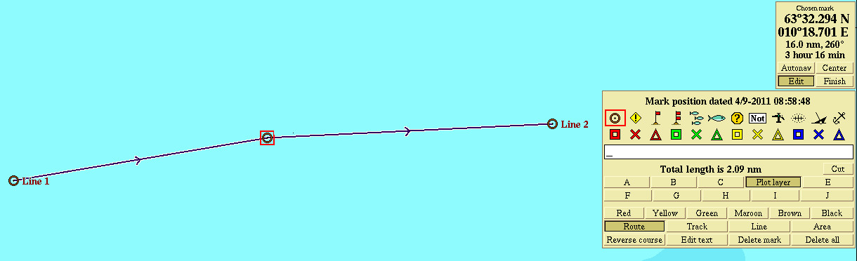
GRIB objects
Import and export data
| Import | Export |
|---|---|
| Software upgrades Olex/Lino | Plotter data (backup) |
| Nokkel files | Depth data (backup) |
| GRIB data | Screenshots |
| Vector chart data | Hardware id |
| Plotter data (from other Olex systems or own backup files) | |
| Depth data (from other Olex systems or own backup files) |
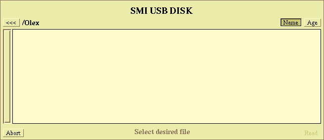
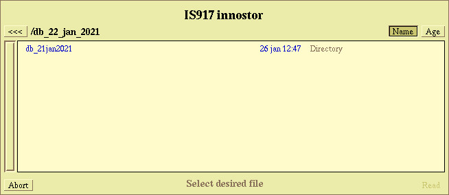
The filebrowser
Open the filebrowser
The filebrowser provides a file managing interface within a specified directory, and it can be used to import, export, preview, rename, edit or delete files on the disc.

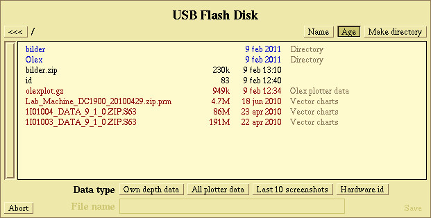
File names have different font colors depending of the type of file.
- Blue font - file directory
- Red font - files ready for import
- Black font - all other files
In addition, some of the files have a sub text showing the file extension.
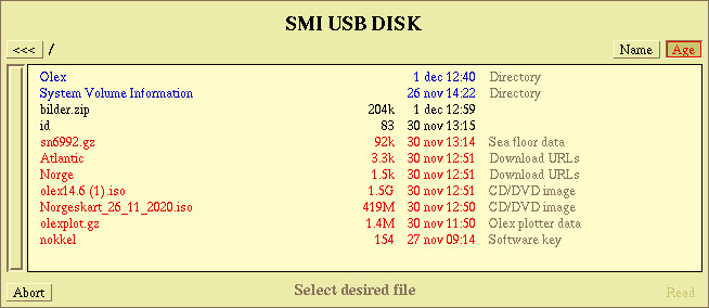
Sorting directories and files
Files and directories can be sorted alphabetically or chronologically depending on the date they were created or modified. Note that file directories have higher priority than single files, and will be listed at the top of the browser window.
Click Name to sort the files alphabetically
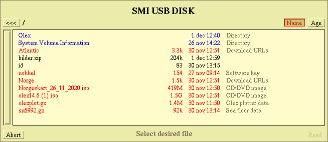
Click Age to sort the files chronologically, the newest file is placed in top of the browser window.
File navigation
Click once on the directory name to access a file directory.
Click once on the arrow in the upper left to go back. The path, to the right of the arrow, shows the location in the file hierarchy.
Create a directory
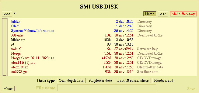
To create a new directory: insert a USB device and click Write to or click Settings → Save data to storage device to open the file browser.

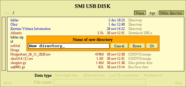
Click Make directory in the upper right part of the browser window.
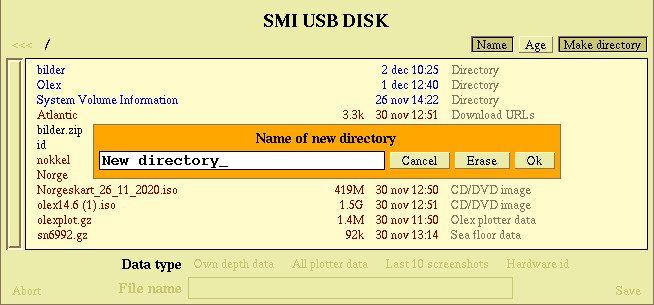
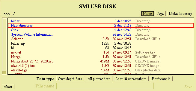
Name the directory and click Ok to save. Click Cancel to close the window without saving, or click Erase to delete the charachters.
Import files
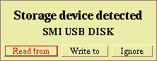
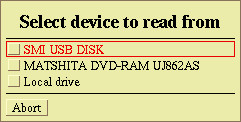
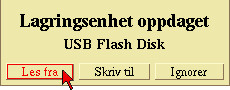
Connect a USB device to one of the USB slots, click Read from to open the filebrowser, or Ignore to close the panel.
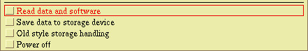
Or click Settings → Read data and software.
Files marked with red are available for import, select files and click Read to import.
Export files
Connect a USB device to one of the USB slots and click Write to to open the filebrowser, or Ignore to close the panel.
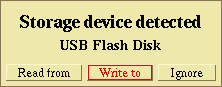
Or click Settings → Save data to software device..
Select the type of file to be saved, Own depth data, All plotter data, Last 10 screenshots or Hardware id.
Create a new directory
To create a new directory, click Make directory in the upper right of the filebrowser.
Name the directory, and click Ok to save.
Copy and move files
Files on the local drive can be copied or moved to other locations. Open the file browser and select the files to be copied by right clicking the filename. The selected files are highlighted in purple.
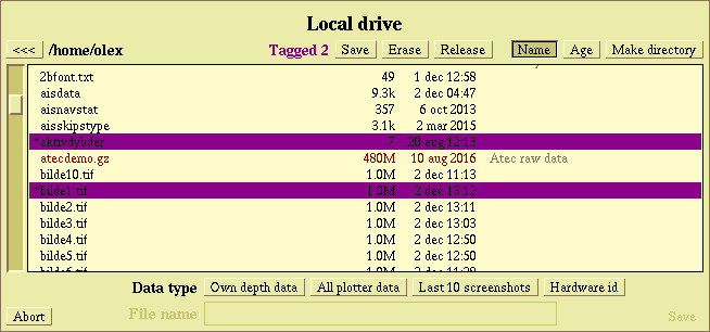
Two new buttons named Erase and Release opens in the upper part of the file browser window. The number of selected files are displayed to the left of the buttons. Click Abort to close the panel, and open the location where to save the selected files. Files will still be highlighted even if the filebrowser is closed. Click Release, and the files are copied into the new location. To move files permanent, go back to the original location and delete the original files.
Delete files
Open the filebrowser and select the files to be deleted. Click Delete and click Yes ,when the warning "Beware! Do you really want to erase files? " opens.
If you confirm to delete the files, a new warning opens, "Files are IRREVOCABLY erased! Shall we continue?", click Yes and the files are deleted. Files that are deleted from the system can not be restored!
Databases
Seabed surveys using GPS and sonar creates a 3D terrain model, based on both measured and calculated depth values. All seafloor data are stored in a depth database. The data can be processed or modified later, errors and suspicious values can be removed, and the data can be imported or exported to other systems.
Shared Olex-data
Users may voluntary submit their depth data to Olex, where the data are processed and stored in one large database. This database is available for all Olex users worldwide, who agree to share their own depth data. The shared database is updated at least once a year, and by submitting own depth data, users will have access to a regularly updated database.
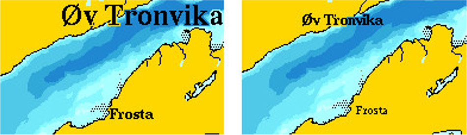
Own depth data
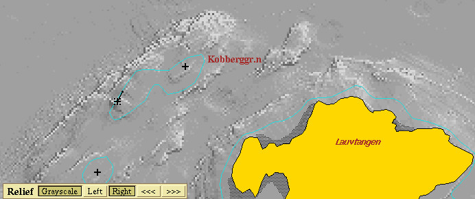
"Own depth data" are data measured by each Olex user. This data will be stored in the database which is set active at the time. Select "Boxes" in the right of the top meny to view all dept values, own depth data are viewed in orange. Data from the shared database are viewed in purple.
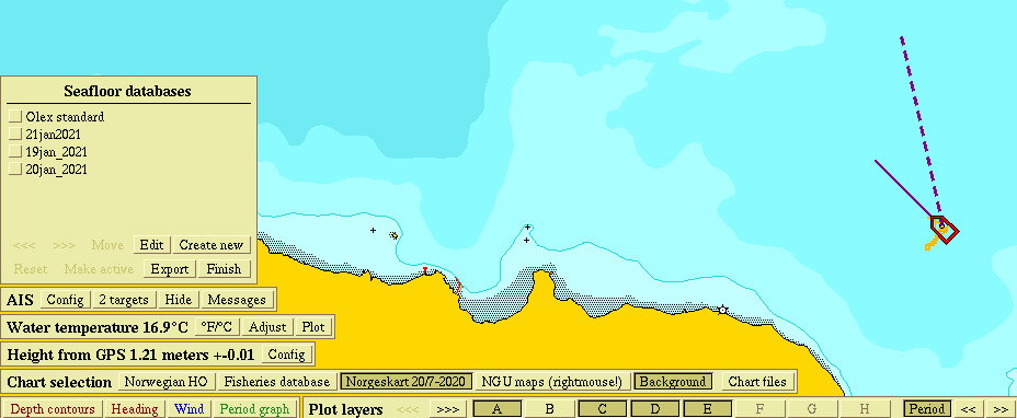
Database panel
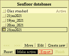
Databases can be easily created, deleted, imported or exported from the Seafloor databases � panel. To open the panel, click on Layers → Manage seafloor databases. The panel has several functions and a list of existing databases. Default database for the installation is Olex standard, but up to 999 new databases can be created by the user.
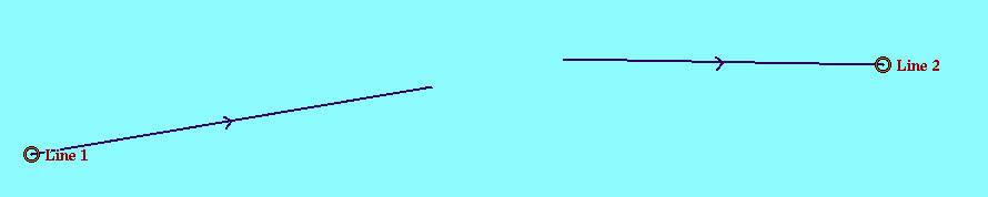
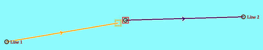
Visible and active databases
A database can be set visible and⁄or active.
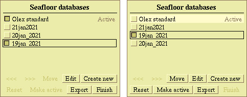
Visible database
A database is visible when the stored depth data are displayed on the screen. Click once on the database name to select, a black frame around the name indicates which database is visible.
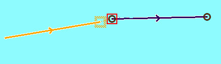
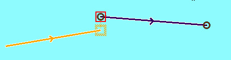
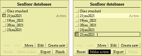
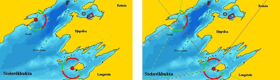
Active database
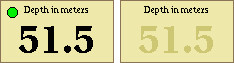
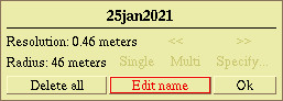
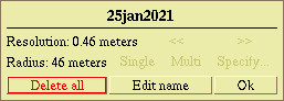
One database is always active. All measured depths are calculated into the active database. To make a database active: select by clicking on its name in the list and then Make active, which is now blinking. A message appears: "Do you really want to shift bottom calculation over to XXXX?". Confirm by clicking Yes. To exit without any changes click No or wait until the red bar has reached the end.
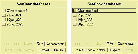
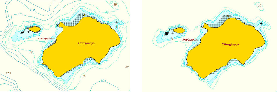
It is possible to set one database visible, and another database active at the same time. I.d data from one database can be viewed for survey, while measured data are stored in another database at the same time.
In the left picture Olex standard is active, and 21jan_2021 is visible. In the right picture, Olex standard is set as well as active and visble database.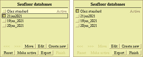
Organizing databases
If there are several databases available, it is useful to organize them so frequently used databases are moved in top of the list. Highlight the database and click Move to move it one step further up.
Create a new database
Click Create new, and a panel opens at the bottom left of the screen. Unless a name is set by the user, the database is named with today�s date. Resolution and calculation radius will be copied from the settings of the visible database, but can easily be set manually.
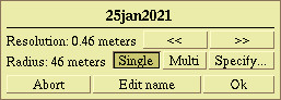
Setting parameters
Select Single if the system is connected to a single beam echosounder or select Multi if connected to a multi-beam echosounder. The system will suggest settings for Resolution and Radius, it is recommended to use the default settings for best results. Parameters can easily be adjusted to the most appropriate value. Resolution determines the level of detail on the depth chart. By changing this value, the dimension of the depth boxes changes. The resolution can be adjusted from 0.06 meters up to 50 meters, by clicking the arrow keys. Radius specifies the radius of the area calculated around a vertical ping. The radius is directly dependent on the resolution. (100 x dimension of the depth box). Click Specify to change the setting for the radius, the resolution will change accordingly. If you select an exceedingly high resolution, it may result in "holes" in the map. By using a low resolution, the radius will be exceptionally large, and large amounts of data must be processed. A lot of system capacity will be spent processing data, and the system may slow down.
Modify an existing database
After a database has been created, only the name can be changed. Highlight the name and then click Edit.
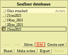
Delete a database
Exept from the default "Olex standard" any database can be deleted, when it's not active. Highlight the database name, click Edit and Delete All. A warning appears: "Do you really want to remove depth database 'xxx'?". Click Yes to delete, or No to cancel.
Export a database
A complete database, with its name and settings intact, can be exported, saved to a storage device and imported to another Olex system.
Highlight the database to be exported, and click Export. A panel with available storage devices opens. Select a location by clicking the name of the device. The filebrowser opens, and Olex will suggest a name for the new file. The name will be of the form "db_xxx" where "db_" is short for "depth database".
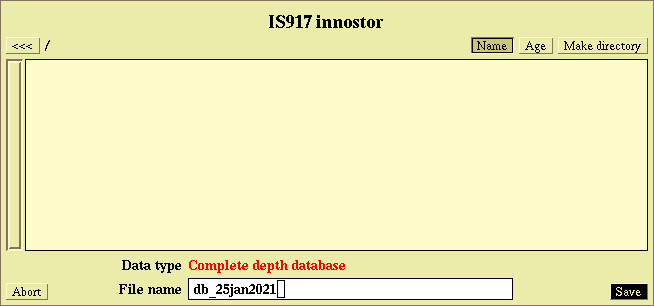
Click Save to export the database, and confirm by clicking Yes, when prompted "Complete depth database - do you really save?". A green panel with the text "Exports dybdedatabase 'xxx ' " is displayed while the database is stored, note that this may take some time as some databases may contain large amounts of data.
Import a database
Open the Filebrowser by clicking Settings → Read data and software, or connect a USB device.
Click on the filename to open the database directory.
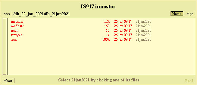
Highlight the files by clicking on any of the files.
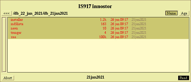
Click Read, and confirm when asked "�xxx - do you really want to read?". The database will be added to the list when the import is ready.
Navigational charts
Both official electronic vector charts - ENC'er, and commercial navigational charts can be used in Olex. The charts can either be purchased from local suppliers or directly from the chart provider. In some contries the navigational chart s are free to download.
Electronic navigational charts are available in different formats, Olex uses the following: S-57 is an international standard for navigational charts that is approved by the IHO - The International Hydrographic Organization. Most of the chart types used in Olex, follows the S-57 standard. The charts can also be encrypted. S-63 is a standard for encrypting and securing electronic charts. Charts using this format consists of an encrypted chartfile, and a permitfile. In addition, navigational chart systems are divided into official and commercial navigational charts. Official charts are the electronic navigation charts recommended by the authorities. The charts are updated regularly, and are the best and most accurate charts for navigation.This charts usually consist of a set of base-CDs that contains the map files, and these charts are updated regularly. Most official charts are sold as subscriptions, and the charts must be deleted from your computer when your subscription periode expires. Commercial charts are updated sporadically, and may therefore have slightly less accuracy. The commercial charts are often a better option when it comes to price.
Charts types
Norgeskart
PRIMAR and IC-ENC - International Centre for ENC's
PRIMAR is a Norwegian regional coordination center that is operated by the Norwegian Hydrographic Service, and provides official charts worldwide. IC-ENC is an international center for official electronic navigation, and provide official charts worldwide.
Chart World
Provider of both official and commercial charts worldwide.
NOAA
National Osceanic and Atmospheric Admistration is an american organization that provides official nautical charts for the U.S. and some other parts of the world. The charts can be downloaded for free, but the rights for use are regulated by NOAA.
Norwegian Fisheries Database
The Norwegian Fisheries Database is created by the Norwegian Mapping Authority. The charts are available from the provider.
NSKV
The charts are older electronic navigation charts for Norway, and are no longer updated. The maps can be purchased by contacting Olex.
SOSI
SOSI - �Samordnet Opplegg for Stedfestet Informasjon� (�Coordinated Arrangement for Localized Information�) is a data format developed by the Norwegian Mapping Authority. SOSI maps are not intended for navigation, but can be used for additional information where there are no charts or where navigational charts are not good enough. I.e. surveys done in lakes or rivers.
GeoNames
Geonames is a geographical name database that contains names throughout the world. The database is pre-installed in Olex and can be used in addition to the chart names.
Installing charts
The maps can be purchased either from distributors or directly from chart provider. Remember to save the original chartfile and permit after installing the charts! When updating Olex version it will sometimes be necessary to reinstall the chart files.
Encrypted chart systems
Encrypted chart systems usually consist of one or more chart files, and a permitfile for installing the chart files.
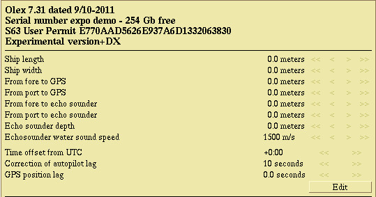
Permit file
All Olexsystemer has an unique S-63 User Permit to be found in the Settings menu.
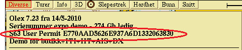
This is an unique ID that identifies your computer, and which must be provided to the chart provider to receive the necessary permit file.
Chart files
Chart files can either be downloaded from the chart providers website, or chart files can be sendt by mail depending on the chart providers routines. Map files can be .iso or .zip files. Iso files are files that represents a copy of the complete file system, usually a CD. File permissions and other metadata will not be lost in the transfer of the iso files. Zip files are files that are compiled and compressed to save disk space.
Installing charts
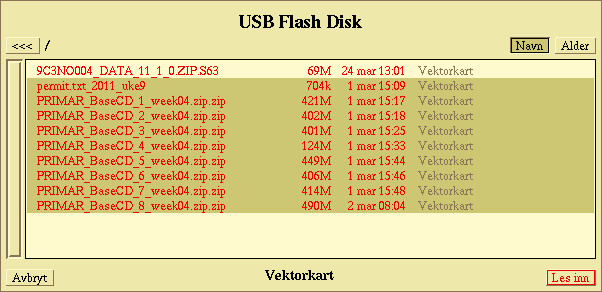
Save the chart - and permit files to a memory device, and connect to the machine. Installing chartfiles in Olex is done in the same way, independent of the chart system. Clich Read from and select the USB device to open the Filebrowser.
Highlight the chart - and permitfiles by clicking at them, and then click Read. Confirm when asked "Vector chart - do you really want to read? ".
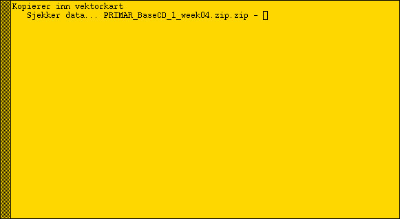
The computer will read the permitfile first and then continue with the chart files. The yellow status window shows the installation progress, and eventually any error messages if there are problems with the install.
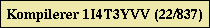
Once all the chart - and permitfiles are read the machine starts comliping the charts. Each of the chart areas consists of several smaller cells, and the progress is shown in panel at the top left.
While the chartfiles are compiled, a button with the chartsystems name is added to the button row down in the left corner of the screen.

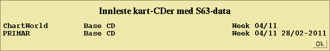
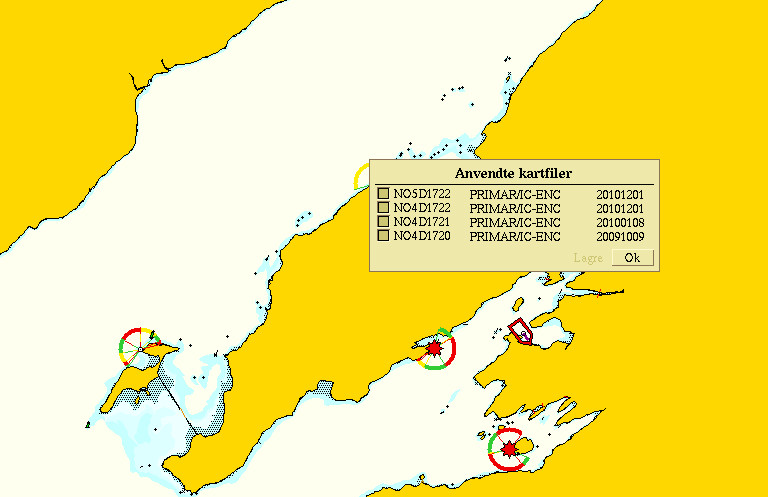
The button CD-index opens a panel with an overview of the base-CD�s that are installed.
The button Chart files opens a list of which chart cells that are used in the visible screen. The charts can be switched on and off by clicking on the check box to the left.
Updating charts
When a chart update is available, install the chart file to thesystem in the same manner as the initial installation. Some updates may require a new permit, this is available at inquiry to the chart supplier.
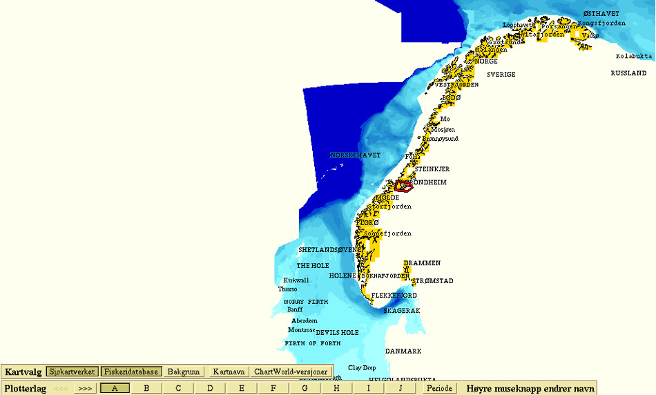
Charts overview
The row Chart selection shows an overview of charts that are installed on the machine.

The charts can be turned on and off by clicking on the button for the respective chart system. Background turns on and off a chart showing the landcontours. This chart is preinstalled on the machine.
GeoNames turns on and off the display of the name database. Chart files displays the chart files used on the visible screen. CD index shows the base CDs that are used. ChartWorld-versions displays an overview of the chart world-charts that are installed.
Deleting charts
To delete charts, click Layers → Chart catalogue → Uninstall vector charts. Choose the chart to be deleted.
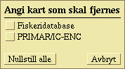
And answer Yes to the question of "Beware! Do you really want to remove the vector charts? " Answer Yes to the question of" This will REMOVE charts and permitfiles! Shall we continue? ". A red status window opens and shows progress in the removal of the charts.The window closes again when the charts are deleted.
Using charts
Visulization
The chart line down in the left shows which maps are installed on the machine.

The charts are turned on and off by clicking the button the respective og the chartsystems. The background chart and GeoName are installed on the machine by delivery. The charts consist of layers with different levels of detail. When zooming out or in, the view changes automatically between the different layers. If the function Layers → Auto chart selection is turned off, a button row opens at the top of the screen corresponding to the different layers. It is possible to select which layer - detail level to be displayed.

Other chart features
Hide depths
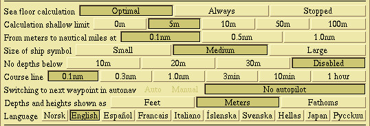
In the Settings menu there is an option for hiding depths of more than 10, 20 or 30 meters. Only depths that is shallower than the selected number will appear on screen. Click Setting → No depths below 10, 20 or 30 meters. To always see all depths choose Disabled.
Small text and symbols
If the texts and symbols are large in relation to the chart view, click the Layers → Small texts and symbols.
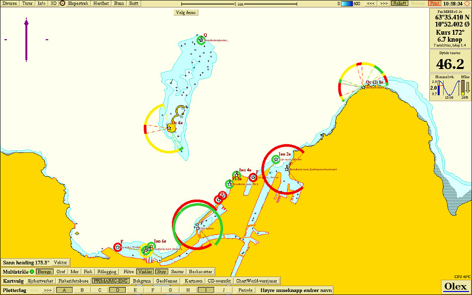
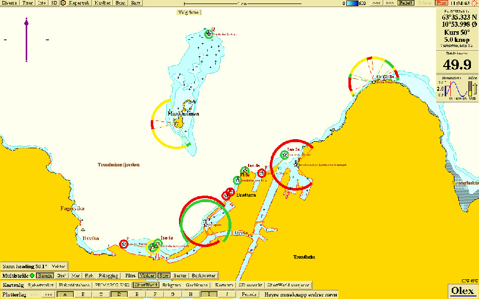
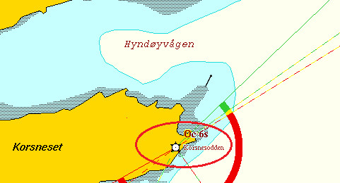
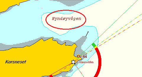
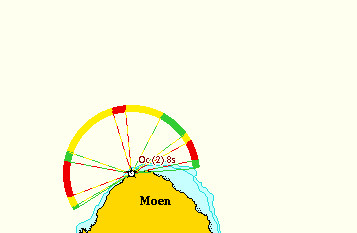
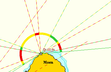
Animated lights
For easier navigation, lantern symbols are made that changes color according to which sector the ship is in. The symbol will flash in accordance with lights flash characteristic, if the data can be found in the map. Only lights that are believed to be visible from the ship will be active. Activated the function by clicking Layers → Animated lights. To see the light sectors and their sector lines, the function Lights and light sectors , and - their sector lines must be enabled.
If the machine does not receive signals from GPS, all lights in chart will be flashing.
Grid lines
Click Layers → Grid lines to turn on a grid showing longitude and latitude.
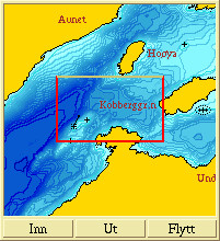
Overview Map
When the map is very zoomed in, it can be convenient to use the overview map. Click Settings Show movable overview map.
Vector chart data
The Layers menu lists the various functions related to vector charts.
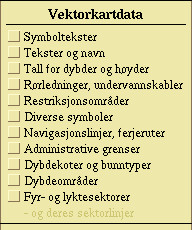
Symbol texts - turn off and on texts that are associated with symbols for the name of light houses, floating buoys, poles and etc.
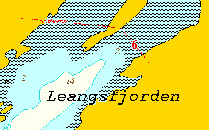
Texts and names - turns on and names in the map, like names of banks, fjords and grounds.
Depths and elevations - turn on and viewing of depths and heights.
Pipelines, subamrine cables - pipelines and submarine cables are displayed with dotted lines.
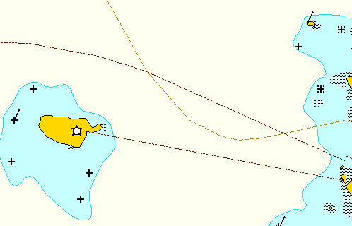
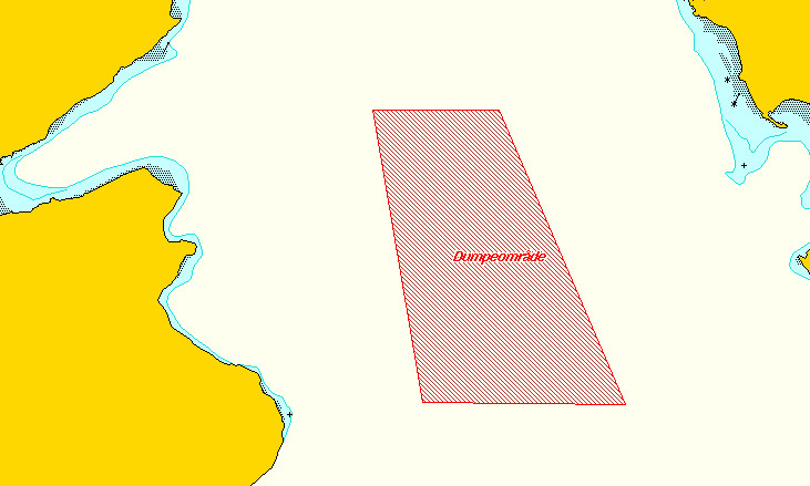
Restricted areas - Showing areas that are subject to an order of restriction, it can be dumping areas or military practice areas.
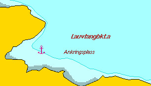
Various symbols - Turns and other types of symbols, like anchorages, shipwrecks or other obstacles.
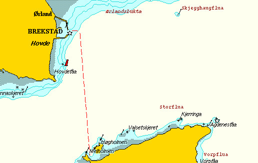
Navigation lines, ferry routes - Displays the ferry route with dotted lines.
Economic and political bourders - like port limits,municipal boundaries and other boundaries.
Depth contours and seabed types - shows the depth contours in addition to any depth numbers.
Depth Areas - shows the depth areas on the map with colors instead of depth contours.
Lights and light light sectors - turn on and off display of lights and sector lines.
- and their sector lines - shows the corresponding sectoral lines.
Seafloor mapping
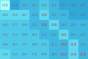
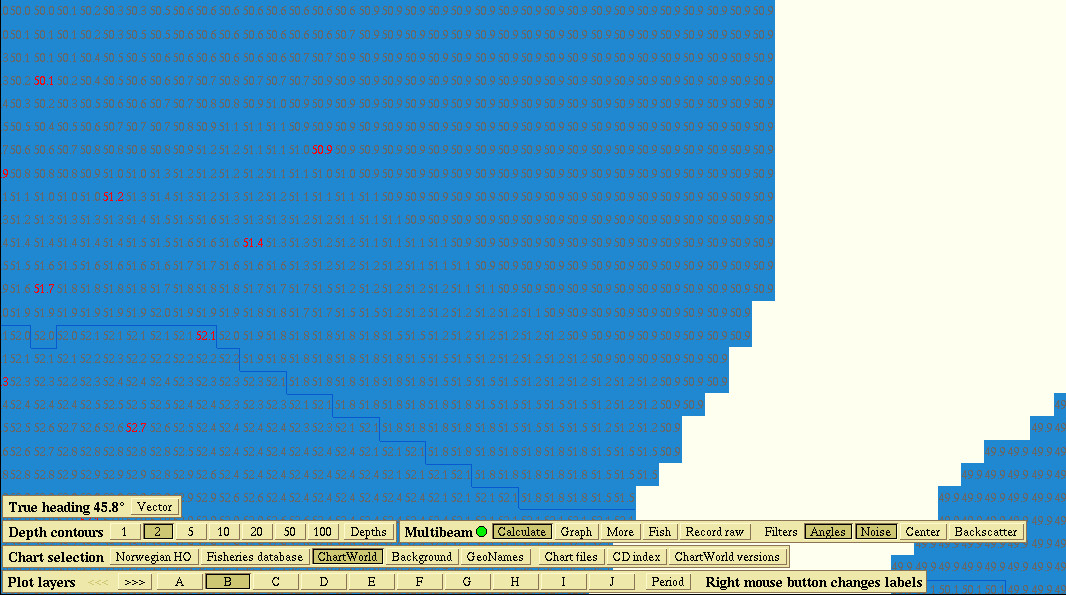
When Olex receivs signals from GPS and echo sounder, the system will automatically start calculation of seafloor maps. Position, bottom- and possibly hardness data, if available, are stored in boxes that are either measured or calculated. Depth data may come from various sources, such as single-beam echo sounder, echo sounders with hardness - ES60 , and multi-beam echo sounders. Data can be imported and exported, via backup, data export, raw-data files and depth databases. The seafloor map can be displayed in different ways, with contours, relief, bottom hardness, bottom zoom and 3D. Any errors that occurs during the surveying can afterwards be removed in different ways. The earth surface is divided into small squares, called depth boxes. Each box is 5x5 metres, unless a different resolution is chosen. This resolution is chosen to match the position accuracy of a conventional GPS. If a more accurate GPS is connected, the resolution can be changed. A depth box can contain either a measured or a calculated value. When the echo sounder receives a value, the value is stored in a deep box, and the system will calculate the depth values in a given radius around this. By zooming in, one depth value is displayed in each depth box. Measured values are red and calculated values are dark gray.
Create seafloor maps
Depth data is the basis for the seafloor maps, and may come from various sources.
Single beam echo sounder
To get the best possible result of the seafloor mapping, it is important to set the correct parametres for the sonar depth, sound velocity and location of the depth sounder. In addition, values for the GPS and the boat's geometry must be set. Click Settings � Edit and use the arrow keys to change the values.
Different parametres can be set to optimize the calculation.
Seafloor calculation
- Optimal - performs a quality check before the values are used in the calculation.
- Always - uses all depth values.
- Stopped - turns off the calculation.
Seafloor calculation should normally be set to "Optimal" for a best result.
Calculation limit
Sets the upper limit of depth values to be used for calculation. This should normally be set somewhere between 5 metres and 100metres. appropriate recommendations may be 5m or 10m.
Echo sounder with bottom hardness
On the basis of raw data from the echo sounder, Olex calculates the seabed topography and hardness. This is done based on the seabeds ability to reflect sound, adjusted for factors that may affect the measurements. Without HT-software, the data will be treated as data from a csingle beam sounder, where only the depths are transferred via serial cable. The hardness is displayed with colors. Each color representing a hardness value. Turn on the hardness view by clicking Hardness in the main menu.
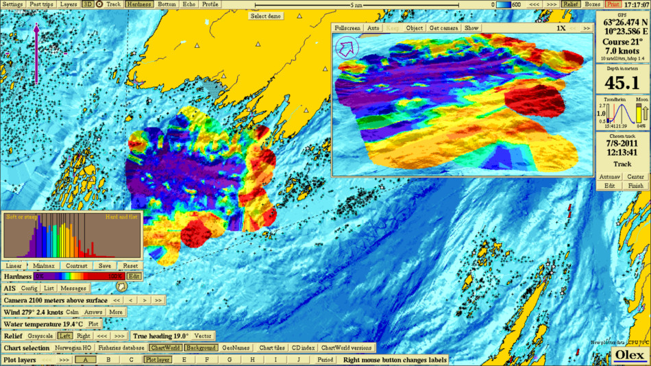
The hardness is expressed in percentage, where 0 % is comp-letely soft and 100 % is maximum hard. The hardness of the last recorded sounding appears in a separate panel to the right. The hardness value is also displayed in the depth flag that appears when the mouse pointer moves around the in the screen.
Multi beam echo sounder
Multibeam echo sounders are used primarily for surveys and seafloor mapping, providing a significantly better accuracy than conventional single-beam echo sounders. On the basis of incoming position- and depth data ,Olex can calculate the seafloor map. Measured and calculated dept data are added continuously to a depth database
Visualization
The self-measured seafloor map can be displayed in different ways, with contours, relief, bottom zoom, 3D, or profile. To turn on and off the seafloor map view, click Layers → Show caclulated seafloor map.
Contour lines
In traditional presentation, the seafloor map, with contours or depth numbers, is displayed on the screen. The seafloor map is displayed in blue tones, ranging from bright blue that means shallow areas, to dark blue that means deeper areas. The colors are allocated from the surface down to a certain depth value, which can be set in the menu bar. All seafloor deeper than this value gets the darkest shade of blue.
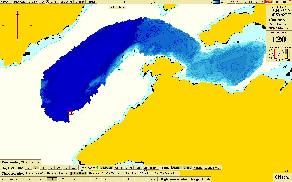
The depth range is set by clicking the arrow buttons on the main menu, minimum depth is 5 meters and maximum depth is 9000 meters.
Equidistance - the depth difference between each contour line, automatically adjusts the selected depth range. The equidistance can also be set manually by clicking on the value in the depth contour panel at the bottom of the screen.
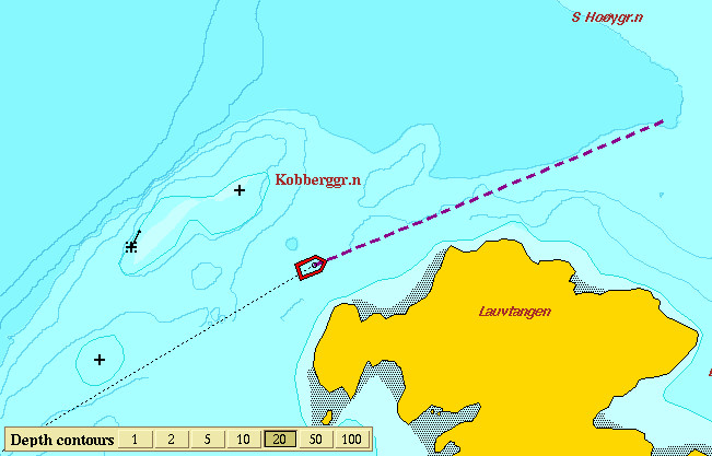
If the map is zoomed in enough, a new button, Depths, is added to the depth contour panel.

By clicking this, the numerical values of the depth of the boxes will be visible on the screen instead of contours. Depths and contours can not be displayed simultaneously.
The map will still have the same colors for the depth areas.
Relief
This function is activated by clicking Relief on the top menu. Depth countours are displayed and visualized by the use of light and shadow. This displays edges and countours, and the detail becomes more visible. A good relief view, depends on if the area has a well-measured seafloor map.
When Relief is activated, a control panel opens in the lower left corner.

Greyscale displays the Olex map in gray colour, with only light and shadow. By clicking Left or Right, you can select the light falling onto the map from the left or right side. This brings out details that might otherwise be difficult to detect. The arrow keys <<< and >>>, are used to increase or decrease the image contrast.
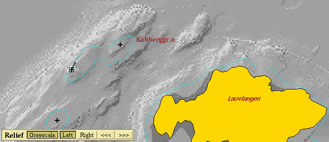
The images displays the same map with relief in grayscale. The first picture is the light in from the left, and the last light coming in from the right.
Bottom zoom
The Bottom zoom function is used to view certain areas in greater details. By activating Bottom in the top menu, the seabed where the depth falls within a certain range, is displayed in details. This presupposes that there are already seafloor maps in the area. Areas without seafloor maps are shown as white. Special colors are used to distinguish the bottom zoom range from the rest of seafloor map. Bottom zoom depth range has an upper and a lower depth limit, centered around a center depth. The center depth is either the depth beneath the vessel, the depth below a mark or it can be set manually. The depth range between each color is adjusted by using the the arrow keys in the bottom zoom panel. By changing the color range, the bottom zoom depth range changes correspondingly.
Bottom zoom has several uses:
- visualization of formations.
- highlight contrasts between depths.
- removal of sounding errors.
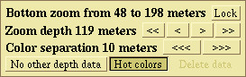
The settings for the bottom zoom range is defined at the top of the panel. A higher color separation, means a broader zoom range. By clicking on the arrows that change the color separation, one will see that the bottom zoom range depends on the color separation. The centre depth is changed by clicking the arrows, << and >> changes the depth by 10 meters for each click, while < and > changes the distance by 1 meter. When the bottom zoom depth range is set, the parameters can be stored for later by clicking Lock. When Bottom is activated later, the previous settings are recalled. If Lock is activated when the panel opens, it means that manual mode was used the last time the bottom zoom feature was used. No other depth data turns off and on all other colors than the bottom zoom colors. Hot colors change the color spectrum from cool blue tones to warm colors.
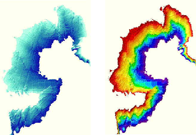
Color separation
15 colors are distributed evenly in the bottom zoom depth range. Each depth range is assigned to one specific color. If the color separation is set to 1 meter, this means that depth areas that have less than 1 m depth difference will have the same color. Bottom zoom range will be 15 meters.If the color separation is increased to 5 meters, the depth areas that varies by less than 5 meters, will have the same color. And the bottom zoom range will be 75 meters. The color distance is adjustable from 0.1 to 500 meters.
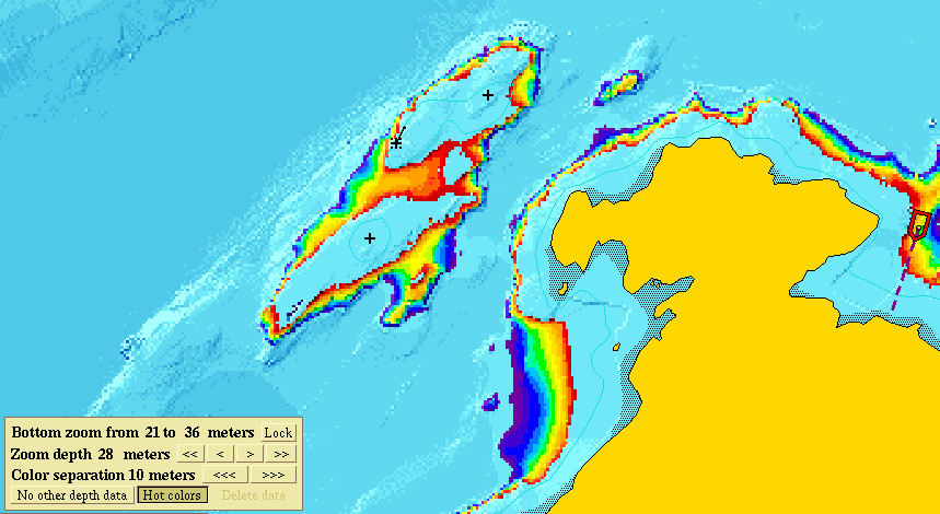
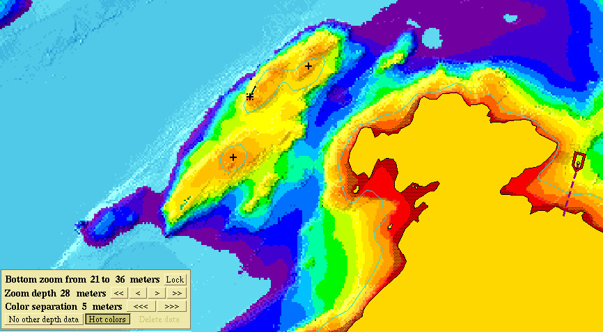
On the first picture is the color space set to 1 meter, on the other photo the color separation is increased to 5 meters.
Zoom depth
The zoom depth can be specified in several different ways.
A mark determines the zoom depth
Select an existing mark, or place a new mark. Click the Bottom button in the main menu. The depth below this mark now determines the zoom depth. If the mark is moved to a deeper or shallower water, the zoom depth changes, and hence the bottom zoom range. After the zoom range is selected, click Lock to keep the setting. The selected mark can then be closed for editing by clicking Finish on the chosen mark panel.
Setting the zoom depth manually
An other way to set the zoom depth, is to adjust it manually by clicking the adjustment buttons on the panel. Notice that the Lock button will be activated automatically when adjusting the settings. The button must be pressed again to return to zoom depths determined by the ship's position, or a mark.
Zoom depth below vessel
Instead of using a mark to determine the zoom depth, and the zoom depth has not been set manually, the depth below the ship at any time determines the zoom depth. This is indicated by that the zoom depth changes constantly, as the ship sails ahead.
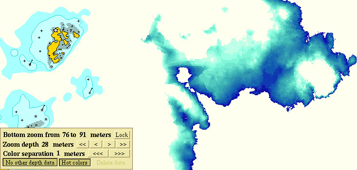
No other depth data
This function turns off the the seafloor map view, displaying only areas with bottom zoom colors.
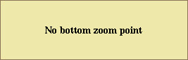
No bottom zoom point
If a mark is placed somewhere outside the measured seafloor map, the zoom depth cannot be determined, and the message �No bottom zoom point� will be displayed.
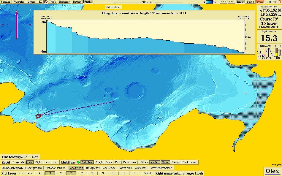
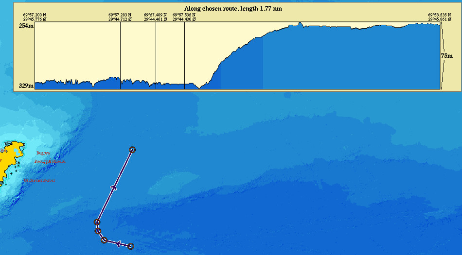
Profile
Click Profile in the main menu, to open a section or profile picture of the seabed:
- Along the ship's course line
- From ship to a selected mark
- Along a selected line object
The seabed profile displays the position for the start and end point, maximum and minimum depth, total height for the entire depth of the profile, and the total length of the profile view. The colors are the same as the colors on the contour lines, or possibly hardness colors.
If the profile from the ship to a mark, or along the ship's course line is selected, the profile will be changing due to the ship�s motion. The view is continuously updated as the coordinates changes. When a profile along a route is displayed, the waypoints are displayed as bars with corresponding positions. The profile view has a fixed size, and the window is scaled to the length of the view. I.e. profiles in the same area may give different views depending on the length of the profile.
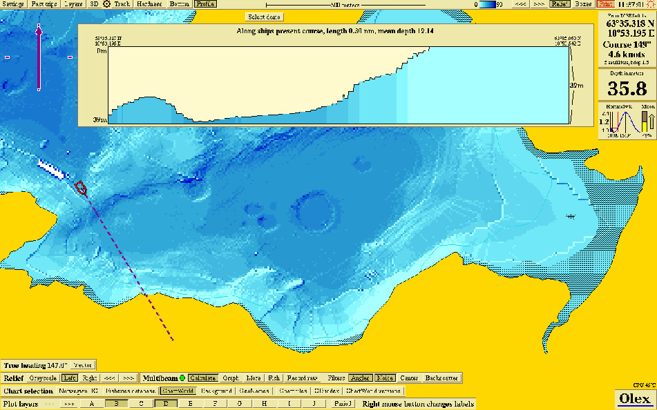
Profile view along the course line
The profile views a cross-section along the vessel's course line, and is updated continuously as the vessel moves forward. The length of the course line can be changed by selecting Settings and select a value for the length of the course line.
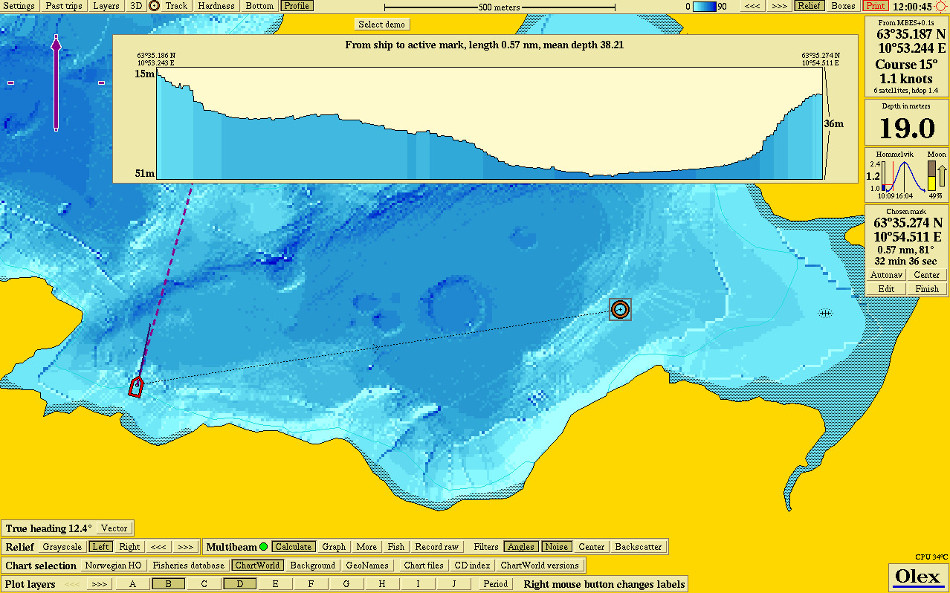
Profile view from the ship to a waypoint
The profile views a cross-section along the line from the ship to a selected waypoint. Grab and placed a new mark, or click on an existing mark. The mark can be moved around and the profile view will be updated continuously.
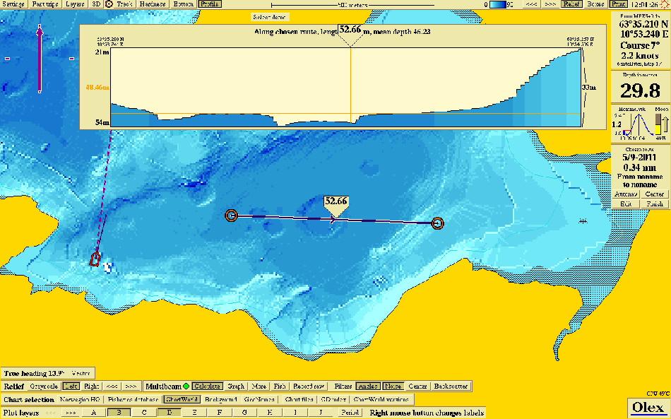
Profile view along a line object
Select an existing line object, or create a new one. The profile along the line object is viewed.

Change coordinates
If a line object is selected, it is possible to change the coordinates by moving the waypoints. The profile changes while the waypoints are moved around in the map.
Create marks in the 2-D map
By moving the mouse pointer inside the profile view, a flag that shows the depth opens both in the profile view and on the map. Click inside the profile view, to place a mark in the 2D view.
Path planning
It is possible to plan routes for piping, cables or other objects on the seabed. The method can also be used to plan for trawl-haul, or find for finding an appropriate place for net and line sets. When the marks are placed, they can be moved around afterwards to find the best location.
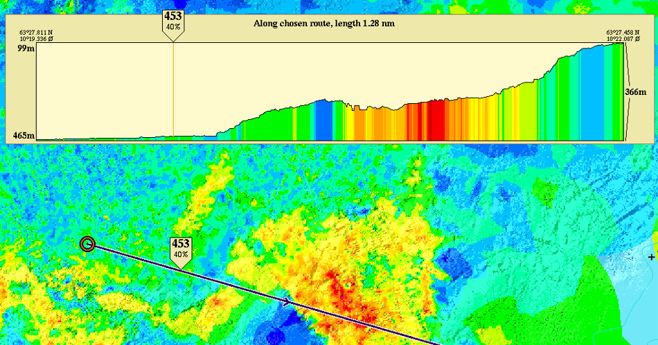
Profile and hardness
The profile can also be displayed with hardness colors.
3D
New perspective 3D
Trips
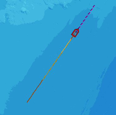
All trips are registered and stored automatically, and can be displayed from the Trips menu. The trips are numbered chronologically, and have a date and a timestamp. Trips data can not be deleted or changed, and can not be exported to other Olexsystemes. A trip appears as a reddish-brown line that is logged in the vessles wake. The color of the line indicates the ship's speed; light color indicates low speed, dark color indicates a higher speed.
Click on Trips in the Main menu to open the Trips panel. The header displays the trip number, date and time. Trips that are registered today, displays the time only.
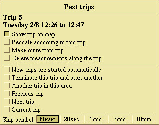
- Show trip on the map - this is the same trip that is displayed in the heading.
- Rescale according to this trip - Scales the map so the entire trip is displayed on the screen.
- Make route from trip - A copy of the requested trip is created, and saved as a new route. The trip will be found in the log and can be displayes as usual.
- Delete measurements along the trip - Deletes all depth measurements along the trip.
- New trips are started automatically - the function start and end trips automatically. A trip is considered completed when the ship has lain at rest over a certain time. A new trip is started automatically when the ship starts moving again.
- Terminate this trip and start another - ends the current trip and start a new trip immediately. The feature can be used even if the function "New trips start automatically" is turned on.
- Another trip in this area - browse the saved trips recorded in the area of the screen. Press the button repeatedly to see all tours in the area.
- Previous trip and Next trip - scrolls back and forth. Then select View trip on the map and Scale the map so the whole trip is to see the trip on the screen.
- Current trip - Displays the last trip.
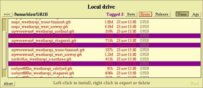
GRIB
The GRIB module downloads and displays weather and other information from the internet. Files in GRIB format contains weather data like wind, currents, waves, air-pressure and precipitation, among others. Both historical and forecast data can be downloaded to Olex. Weather data are displayed with arrows, colors, graphs and animation in Olex.
- See present weather at a particular location.
- Forecast for a spesific location ahead of time.
- Weather prognoses as the vessel passes different locations according to speed.
GRIB also supports download of various types of public information from BarentsWatch, like fishing facilities, maritime borders and restricted areas, in the form of volatile plotter objects.
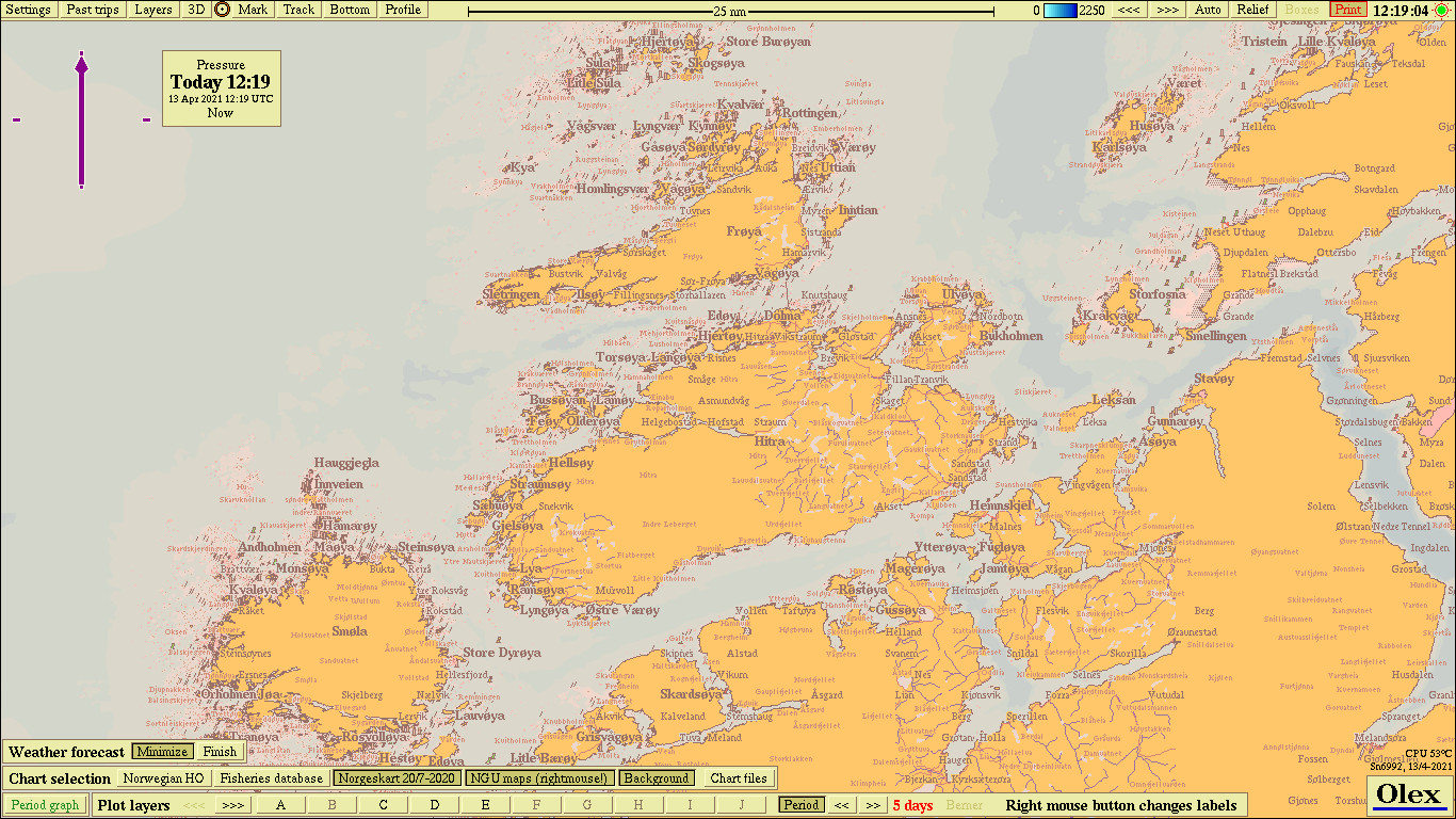
The Weather forecast panel
The Weather forecast panel is opened by clicking Settings → Weather forecast
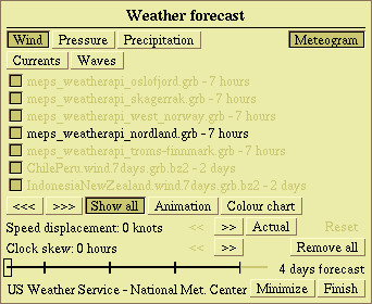
In the upper part of the panel there are a number of buttons where one can choose what kind of weather data to be displayed - wind, pressure, precipitation, ocean currents or waves.
Wind
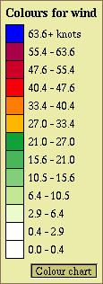
Arrows symbolizes wind direction and speed. The color scheme is inspired by the Norwegian weather service yr.no and shows areas with similar wind speed.
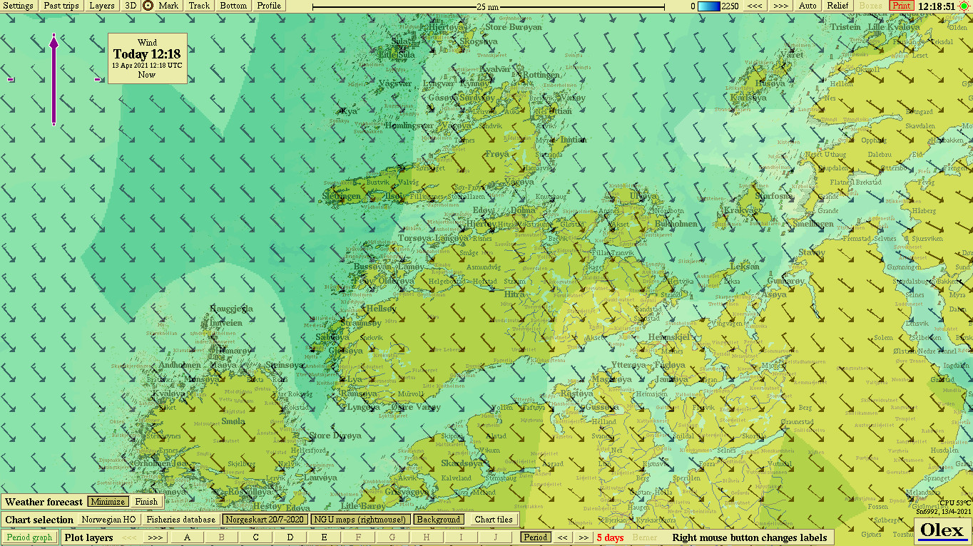
Colour chart opens a table that shows the relationship between wind speed and colour.
Another click on Colour chart closes the view.
Pressure
The colored fields shows areas with approximately the same air pressure.
Colour chart opens a table that shows the
relationship between air pressure and color.
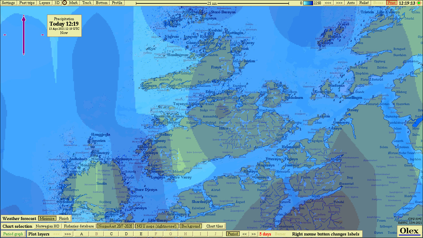
Precipitation
The colored fields shows areas with approximately the same precipitaion.
Color chart opens a table that shows the
relationship between precipitation and color.
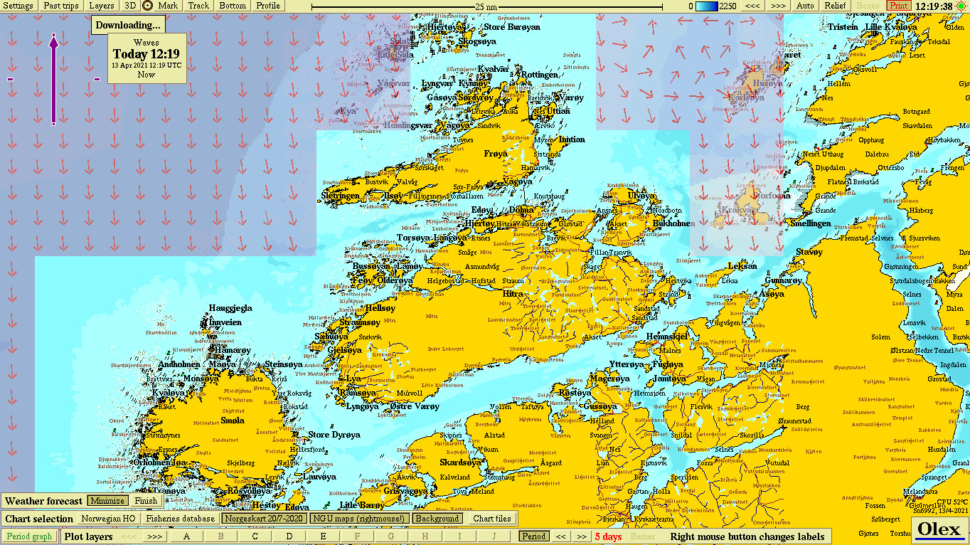
Waves
The wave arrows symbolizes the direction and height of the waves.
The colored fields shows areas that have approximately the same wave height.
Colour chart opens a table that shows the relationship between wave height and color.
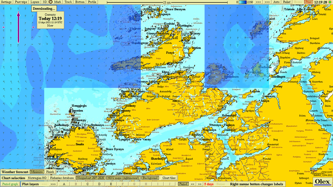
Currents
The arrows symbolizes the oceanic current�s direction and strength.
The colored fields shows areas with about the same current.
Colour chart opens a table that shows the relationship between strenght /velocity and color.
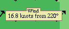
When Weather forecast is selected, the mouse pointer will have a small pop-up panel displaying the type of weather data and the exact value of wind, pressure, wave height or current and direction at the point where the tip of the arrow touches.
Weather forecast and meteogram
All the downloaded weather files are displayed in the list. Each file contains weather for a particular area, and can be turned on and off by clicking the shaded box to the left of the file name. Weather files, currently visible on the screen, are highlighted. Browse through the files by using the arrow keys, left or right, in the bottom of the file menu. Weather files are downloaded from different websites and the respective files are updated by the provider at specific time intervals. Therefore, a weather file may be several hours old when downloaded. The age of the data file, i.e. how many hours since it was created or updated, appears to the right of the file name in the list.
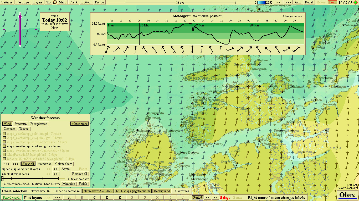
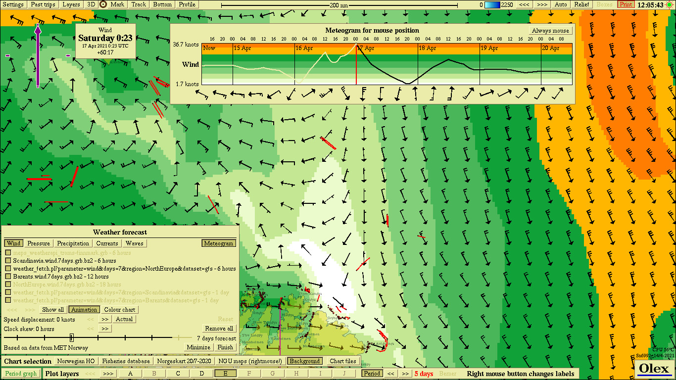
Meteogram
The meteogram opens by pressing the Meteogram button in the upper right of the Weather forecast panel. This graph shows forecasts for up to 7 days in advance, at the position of the mouse pointer. You can also select a particular point / position instead, where the forecast is displayed. The text at the top of the meteogram will then be changed to "Meteogram for the selected point". If a point is selected, but you still want to display the mouse pointer position continuously, click Always Mouse in the upper right corner.
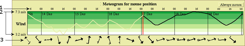
- Weather forecast for up to 7 days - divided in time intervals of 8 hours. The graph shows the estimated variation in wind speed, and the red vertical line shows the time for the forecast. If Animation is selected, the line will move from left to right as the animation is played.
- Highest and lowest estimated wind speed within the current time frame.
- Displays the wind direction at different times ahead of time.
Animation
Clicking Animation will play an animation showing how wind, pressure, waves or current changes over time.
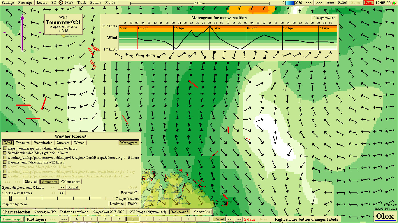
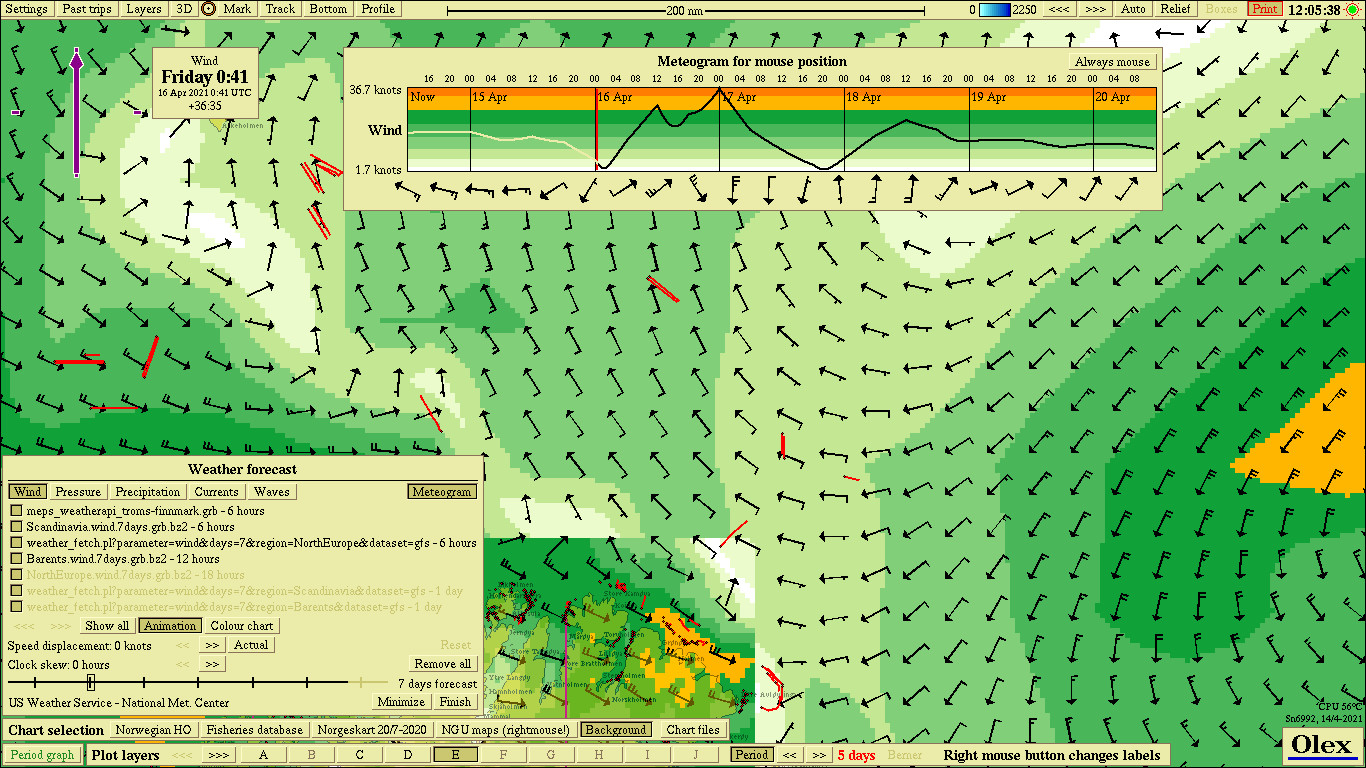
Follow the slider in the lower part of the weather panel to see the time of the animation. The panel in the upper left corner of the map also shows the same time of the animation.
Weather forecast
Weather forcast can be displayed for a specific time, or by how the weather changes as you go at a certain speed. These functions can be activated by selecting either Clock skew or Speed displacement. As mentioned earlier, the weather files downloaded from the different web pages will be updated at certain time intervals. It is an advantage that the data file is as new as possible and by selecting an appropriate time interval for automatic download, you will always have updated weather data available.
Clock skew
Click the arrow keys at the bottom of the weather forecast panel to set the time shift value. This means that if you set the clock skew to 24 hours, the weather forecast will be 24 hours in advance. The slider in the lower part of the panel can also be used to shift the time.
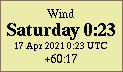
Speed displacement
Speed displacement opens a weather forecast in a circle around the vessel, which extends as far as the downloaded forecast reaches at a certain vessel speed. At the vessels position you will see the present weather, while towards the outskirts of the circle you will see weather at your imaginary position as the ship move at a selected speed. Choose Actual to use the actual speed of vessel at any time. The Clock skew and Speed displacement features can be combined to create a weather forecast for a scheduled trip in a spesific area.
Automatic download
In order to receive continuous updating of the weather files, it is necessary to connect the machine to the internet. This can be done in several different ways, i.e. via ICE or another type of internet connection.
There are several types of downloadable data files:
- weather data
- fishing facilities
- maritime borders
- closed areas
- restrictions
Weather files in "grib" format and other files in plotter data format can be downloaded from different sites like: Yr, Global Marine Networks or BarentsWatch.
URL lists for downloading weather and other data
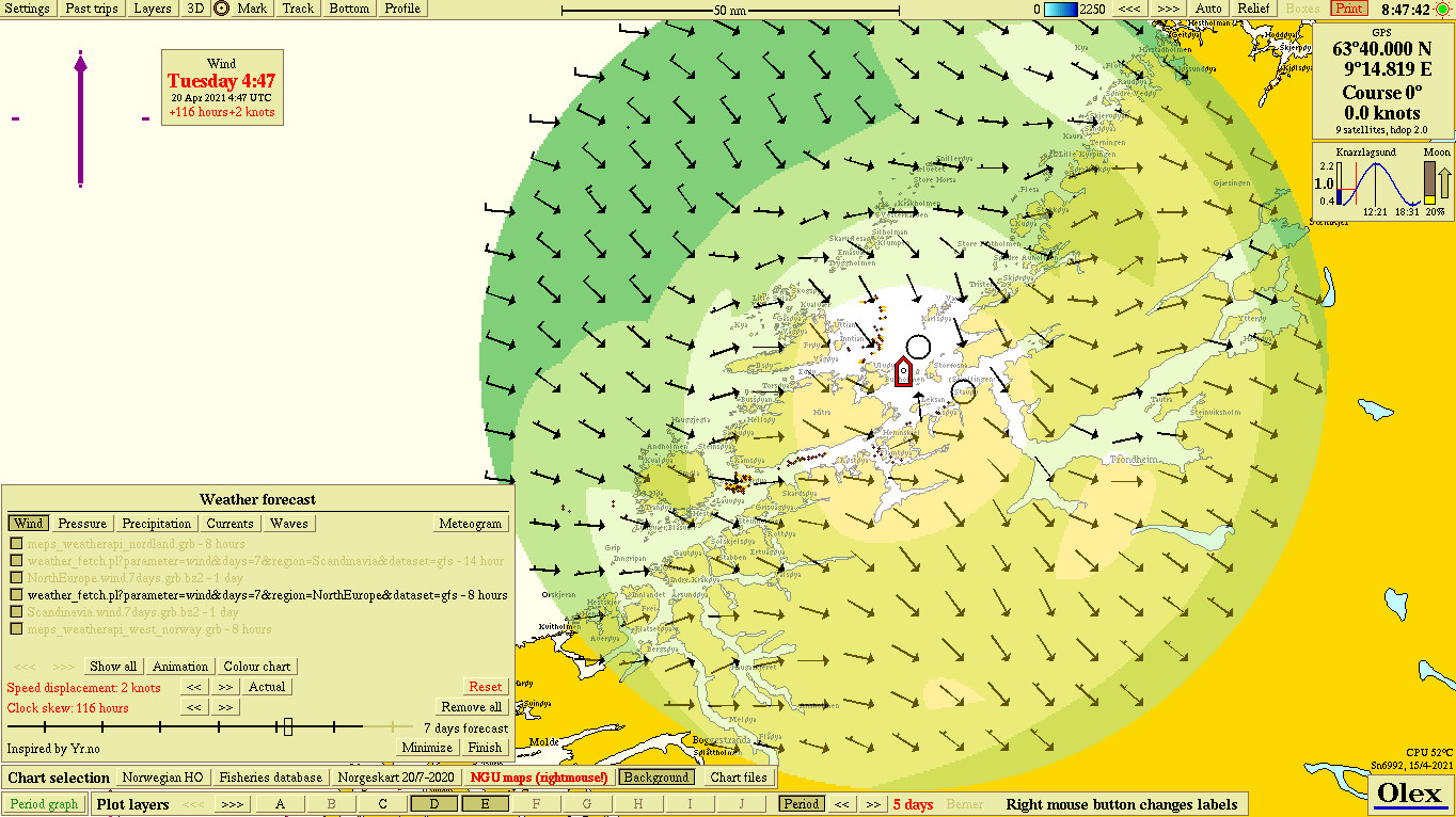
On the Olex website www.olex.no you can find pre-made lists with recommended URLs for downloading weather and other data from various web pages.
These files contains current Internet links that can be used to download data. Right-click on the required files and select "Save link as" to download. Save the files to a USB stick and read them into the Olex.
The Download panel
Click Settings → Downloads to open the Downloads panel. If the URL lists has been successully read in, the URLs will now be visible here. In this panel you can also enter your BarentsWatch user name and password to receive extended information connected to the download of fishing gear positions.
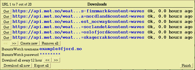
The interval of the automatic download can be set from 0 to 24 hours. Set the interval by using the right and left arrows next to Download all every x hour. Use the Download all now button to download all the files right now. The Export button saves a list of your download URLs as a file, for sharing with others or own backup.
Should you ever need to create a new download URL, in addition to the ones mentioned in the pre-made URL lists, click Create new → ???.

Use the backspace key to clear the characters, enter a new address and click OK.

Manual download to a USB stick
If an Internet connection is not available, grib-files can be downloaded manually from the websites of the various weather services, and read into the Olex via a USB stick. The result is the same as with auto download and can be viewed under Settings → Weather forecast
Reporting of fishing gear
Norwegian authorities wants the fishermen to report the position of their fishing gear to the coast guard. Olex GRIB-module has functions which does this automatically over Internet.
Click Settings → Report gear to open the “Reporting of fishing gear” panel.
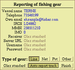
This panel must contain information about the vessel, and also phone number and mail-address. Any red fields must be completed. If you click on Olex standard Olex will use any available information from the ships AIS in order to fill in the fields. Click on the field to fill in or edit the values.
Note! The last four fields should not be edited, but can be left as Olex standard
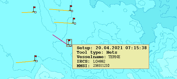
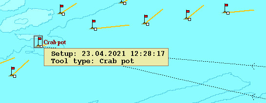
Select your type of gear: Line, Net, Pot or Other
Report a track as fishing gear
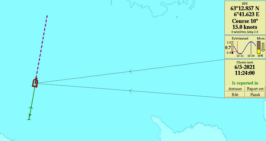
Click on the track you wish to report. In the "Chosen mark" window, click Report in!.
“Do you really want to report fishing gear?“ Confirm by clicking Yes.
The track is now reported. The message "Is reported in" will show in the "Chosen mark" window and the track will flash green and red until it is reported out again.
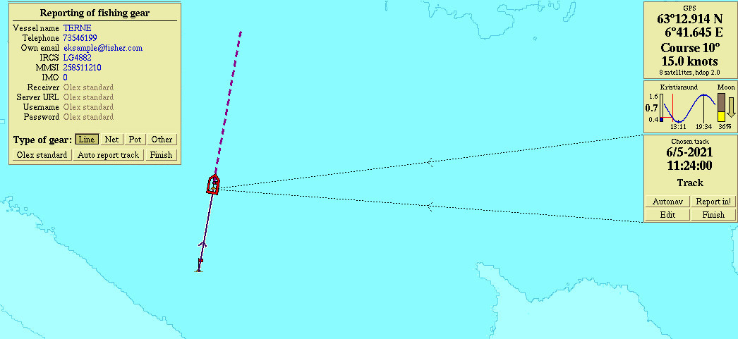
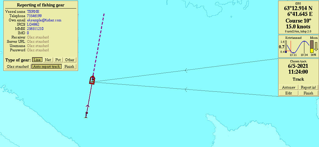
Auto report track
If the Auto Report Track is activated, the fishing gear will be reported when a track is ended. Click Track when the fishing gear is deployed and end the track when finished. Reporting will be done immediately after the track is ended. The track will flash green and red until it is reported out again.
Report out
To report fishing gear out again at the end of fishing, click on the track and select Report out,
“Do you really want to report removed fishing gear?“ Confirm by clicking Yes.
The track will stop flashing, but still be present, now as a regular plotter object.
Extended fishing gear information
To see information about the owner of deployed fishing gear from BarentsWatch, you ned to create an account at barentswatch.no and register your vessel there as well. The username and password from BarentWatch can then be filled in under Settings → Download in Olex to get access to this information.
Even without BarentsWatch log in, type of gear and time of deployment will still be displayed.
AIS
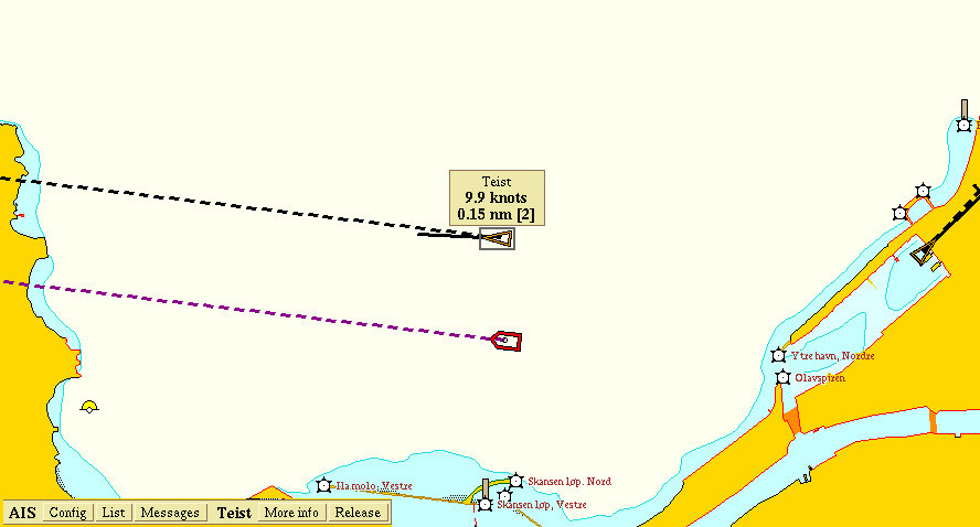
AIS is introduced for safe navigation, and to improve water-borne traffic monitoring. AIS identifies heading and speed of other ships, and its main function is to prevent collision between vessels. Ship information is broadcast over the VHF band, and it will even receive the same information from other ships and base stations. Clicking on an AIS target opens an information box, that displays the vessels name, speed and distance from own ship. The number in brackets shows the time elapsed since the last message from the target was received.
AIS symbols
 Ship symbol, the arrow indicates which way the vessel is about to turn.
 �Sleaping�, the vessel has not been moving for some time.
 The AIS target is about to disappear out of range.
 Active base station.
 The Base station is about to disappear out of range.
AIS targets are identified by its name or MMSI-id.

Clicking on an ais target opens a tag with ship name, course, speed and distance to own ship. The number in parentheses shows the time elapsed (in seconds) since the last message from the target was received.
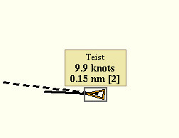
The AIS function panel
Olex systems with AIS, has a function panel in the lower left of the screen. Own ships AIS set-up can be configured here.
The panel has 3 buttons, Config, List and Messages.
- Config - opens a new panel with ship information. The AIS set-up can be configured here.
- List � displays a list of all visible AIS targets within range.
- Messages � broadcasts messages to other AIS targets.
Selecting an AIS target by clicking on it, adds 2 more buttons to the panel, and also the vessels name or MMSI-id.
- More info � displays ship information.
- Relesase � deselects the target.

Configuration
By clicking Config, a panel with own ships AIS set-up opens.
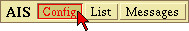
Ship Static Data includes IMO number, MMSI-id, name and call sign.
Voyage Static Data includes information like; destination, number of persons on board, navigational status and type of ship and cargo cathegory.
The information can be replaced by clicking the blue font. A textbox, where to write the new information, opens.

Click Ok to confirm, or click Cancel to abort.
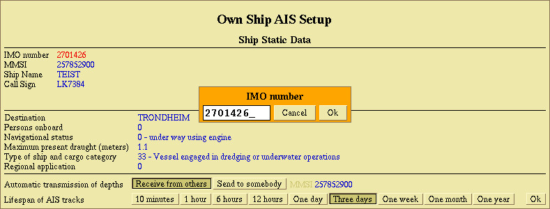
Some of the information are standard sentences that can be changed by clicking one of the arrows until the correct sentence is displayed. Click Ok to save the changes.
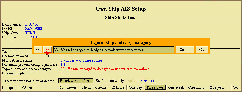
In the lower part of the panel there are 2 rows of buttons. The buttons in the first row sets preferences for depth transfer betweeen multiple Olex systems. The buttons in the second row determines the lifetime of the AIS track. Click Ok to save the changes and close the panel.
AIS targets
Click List in the AIS panel, and an overview of all visible AIS targets within range opens.

The grey check box indicates that an AIS-target is selected, and that the target's info box is open. Click on a name to locate the vessel on the screen. Targets showing the MMSI id instead of the name are AIS targets that:
- have just come within range
- class B AIS targets that can not be identified by older AIS transponders
Names or MMSI id's that are crossed-out, are about to disapperar out of range. By clicking Distance or Name, the list of AIS targets is sorted either by distance or by name.
Sending and receiving messages
Click on Messages to broadcast text messages to other AIS targets within range. A new panel with the heading �Messages� opens. Click on Create message, and a text box opens under the panel.
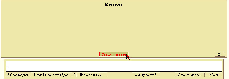
Type the message, and select the vessel from the list of AIS targets. The recipient will appear to the left of the text field as �Send to 'name of vessel'�. Click Send message! to send to the selected vessel.
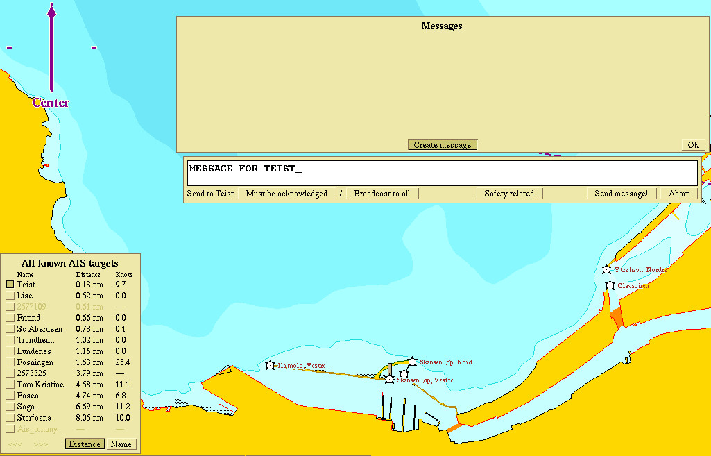
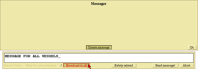
If the message contains a notification of possible danger, click Safety related. The text turns red, indicating that the message has high priority.
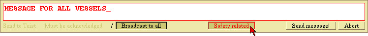
The messages are moved into the upper panel when they are confirmed sent. Status of transfer is shown in brackets in front of the message. When the message is submited, it will disappear from the list.
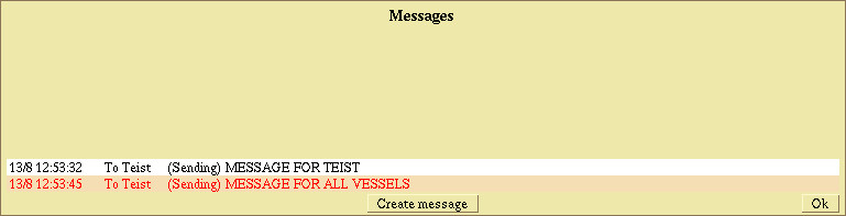
If the transfer fails so that the message can not be sent, the message "** Failed **" appears as the status of the message.
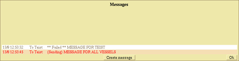
Avoid collision
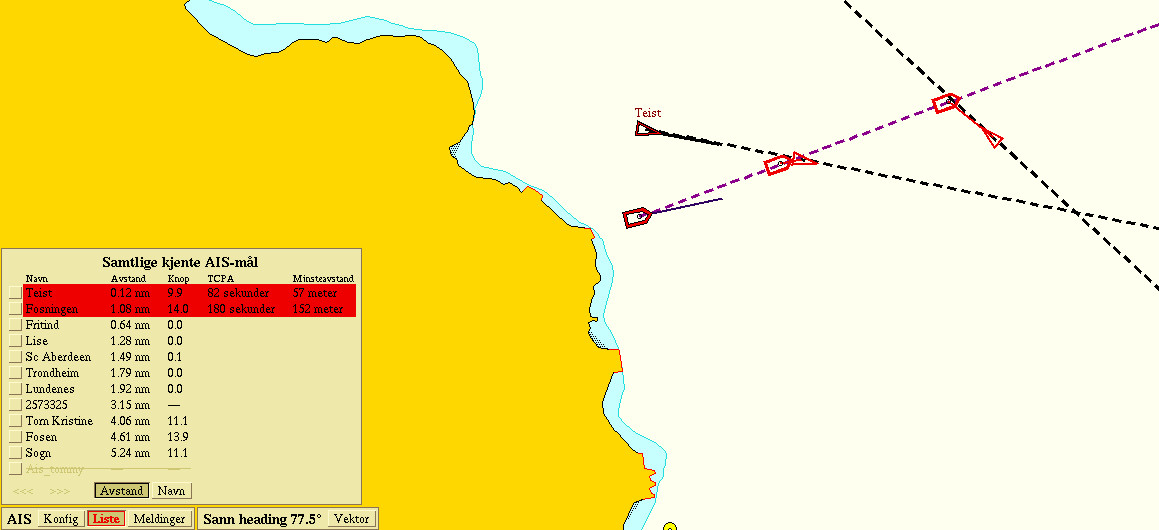
If two or more vessels may come to cross each other's courses, the system will show the possible future situation given the speed and course that the vessels have at the moment.
Warning
The ship symbols turn red if there is less than 2 minutes left for the vessels passing each other closer than 1 / 10 miles (185.2m). The List button on the AIS menu will flash in red, and when the list of AIS targets is opened, the name of the vessels that are within the area will be marked in red. In addition, the column TCPA (Time to Closest Point of Approach) will display the number of seconds to the closest point of approach occurs, and Minimum distance shows the minimum distance between the vessels.Vessels that may be crossing each other's courses with greater distance, is visualized by yellow ship symbols.
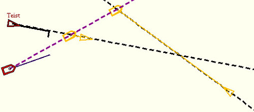
Finding the best course
By turning on Info → Continuous ranging arrow, the cursor can be moved around to try out different courses. The green ships symbols shows that the ship will be passing behind the other vessel.
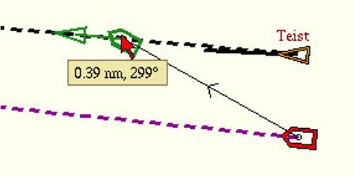
Purple ship symbols show that the crossing occurs in front of the crossing vessel, but with a good safety margin.
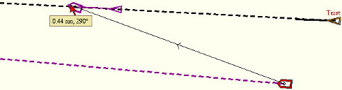
Depth transfer
It is possible to transfer depth values between two Olex systems, so the seabed mapping can be based on measurements from both systems simultaneously. To receive from, or send data to another system, the vessel must be identified with its unique MMSI-id. This can be done in two ways:
Entering the MMSI manually
If the vessel's MMSI is known, click on Configuration to open the panel Own ship AIS setup. Click on the numbers written with blue font to the right of the text Automatic depth transfer.
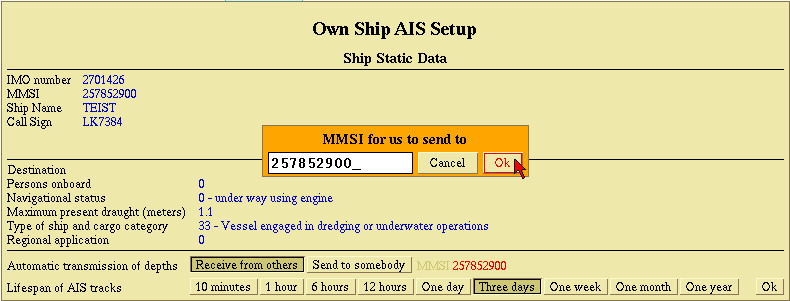
Enter the MMSI-id in the text box that opens, click Ok to confirm. The new value will now be saved in the system.
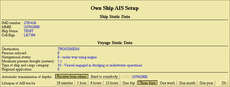
Choose MMSI id from the list of AIS targets
Open the list of visible AIS targets. Then click on the name of the vessel to receive the depth data.
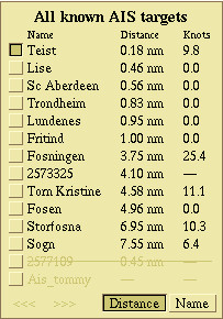
Click More info to open the info panel, and then click Activate as depth receiver.
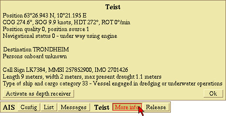
Click Ok to save and close the panel. To follow the calculation process, click Settings → Show calculation progress.
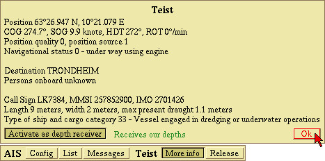
The picture shows the 2 vessels measuring depts, the seafloor map is calcuated continuously on the basis of data from both ships.
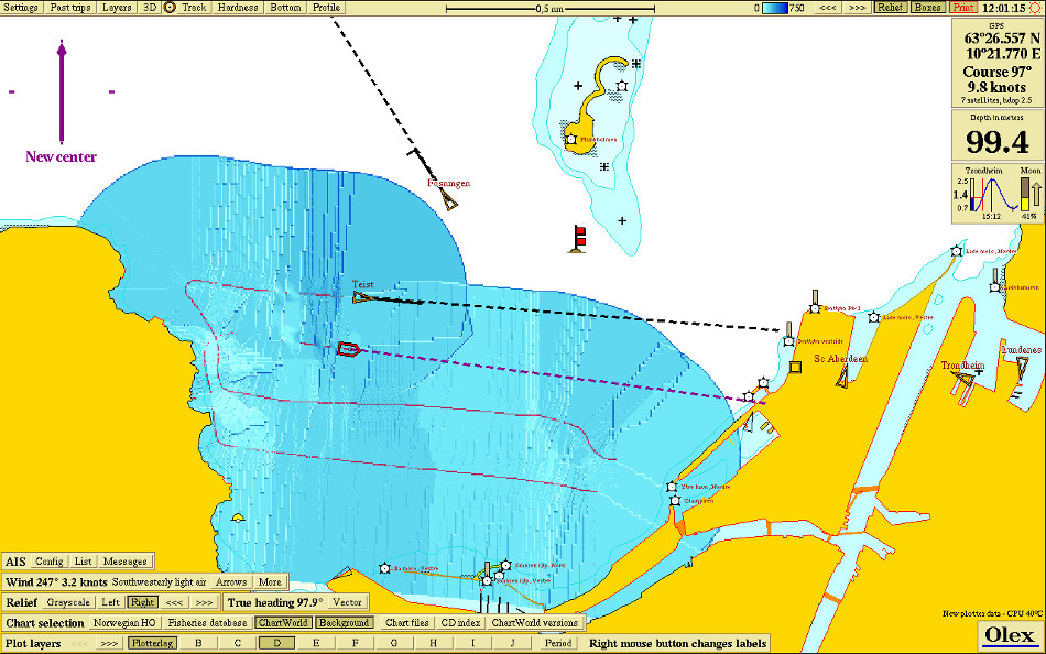
Autopilot
The Autonav function on Olex is designed to provide a clear and intuitive operation of the ships autopilot.
Autonav
The autonav function assists the operator’s control of the vessel by providing steering instructions in the Autonav panel to keep the ship along a selected course. With the ships autopilot connected, Olex will give the instruction directly to the autopilot and help navigate against or along a chosen mark or route.
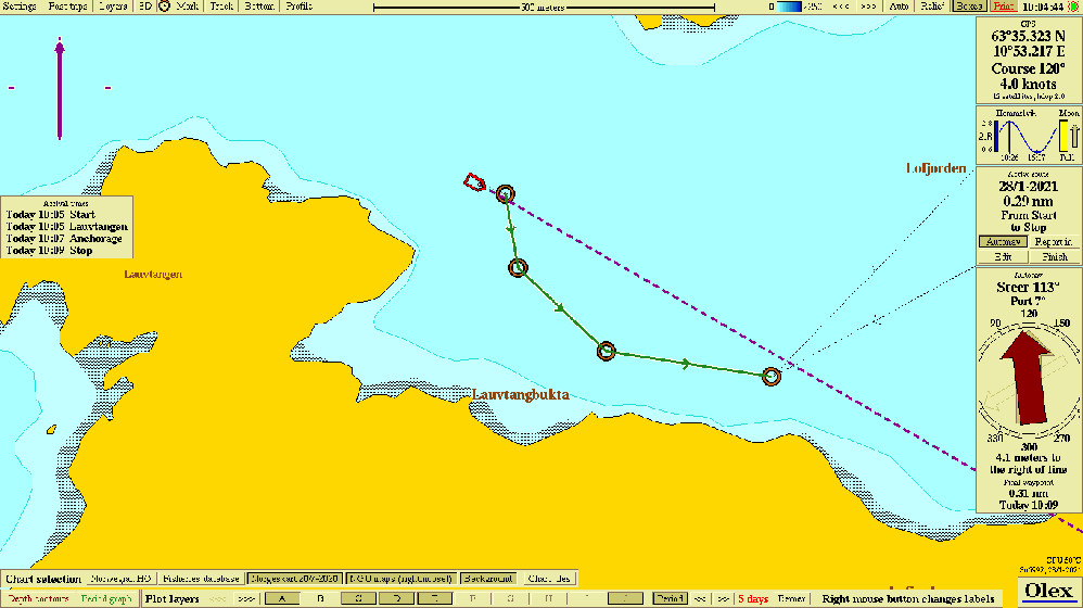
Using Autonav with the autopilot connected to Olex
- Create a mark or line object, and click "Autonav" in the Chosen-mark or Chosen-line -panel.
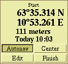
- Click "Yes" to confirm when asked "Initiate Autonav". The autopilot will now recieve signals from Olex and start navigation against or along the selected object.
- The Autonav-panel opens in the right side of the screen. The panel displays a graphical representation of the same messages received by the autopilot.
Using Autonav without an autopilot connected
- Create a mark or line object, and click "Autonav" in the Chosen-mark or Chosen-line -panel.
- Click "Yes" to confirm when asked "Initiate Autonav".
- The Autonav-panel opens in the right side of the screen. The panel displays current course, steering instructions, arrival time and distance. Follow the instructions to steer the ship manually along the set course.
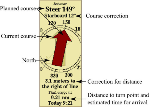
Estimated time of arrival
If a mark is named, or a route has named waypoints, a panel with a list of estimated time of arrival opens when Autonav is started.
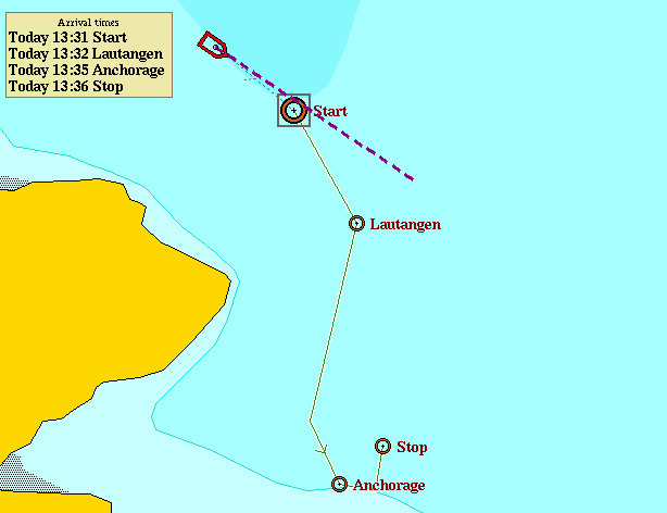
Theese times are calculated continuously, so any change in speed will change the times accordingly. Length of stay can also be taken into account. If a stop is planned, just enter the estimated length of stay after the port name in parentheses: Name of port (10 minutes)
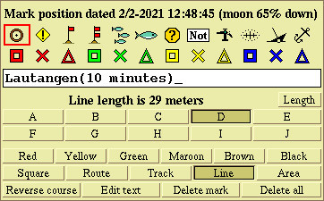
The time of arrival will be changed.
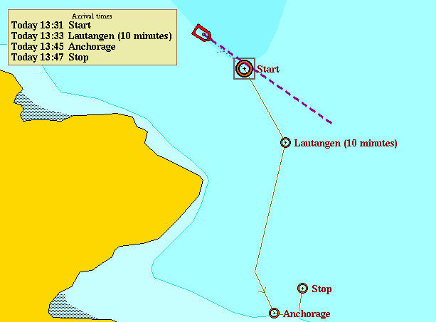
Correction of autopilot lag
Olex Autonav will navigate against the nearest waypoint along a route with several waypoints. When the point is passed, it starts navigation towards the next waypoint.
To keep the best possible course through turn, a correction of autopilot lag can be added in the Olex Settings.
By adding the correction of autopilot lag, Olex will calculate the ship's probable future position in x seconds.
If it is estimated that a waypoint has been passed, Olex starts navigation towards the next waypoint immediately,
keeping the course line as straight as possible. Without correction, the autopilot will calculate the new course after passing the next waypoint.
Depending on the ship, it may take a few seconds or more, to maneuver the ship back on track. The exact number of seconds can be adjusted and testet at sea, until the optimal correction is found.
To add the Correction for autopilot lag, click Settings → Edit.
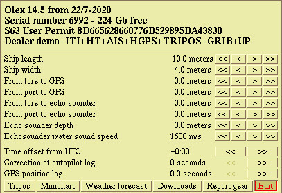
Under correction - too short time correction on autopilot. The ship turns too late and the course becomes unstable.
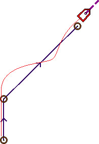
Over correction - too long time correction on autopilot - the ship turns before it should.
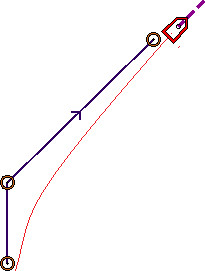
The perfect path - appropriate number of seconds added for delayed autopilot.
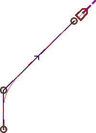
WIND
Vessels equipped with an anemometer have a panel in the lower left of the screen that shows wind- speed and direction, in addition to the meteorological name.
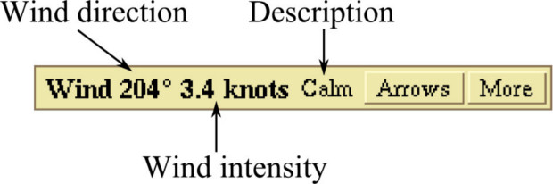
Click on Arrows - two arrows near the ship opens. The red arrow shows the wind direction at the moment, and the green arrow shows the average wind direction for the last 10 minutes.
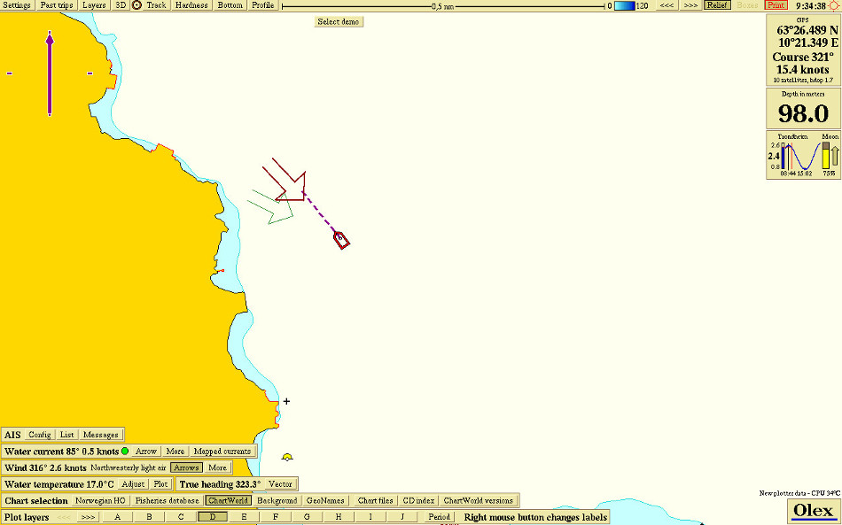
Click More to open a graphical overview of the wind direction and - strength at a given period of time.
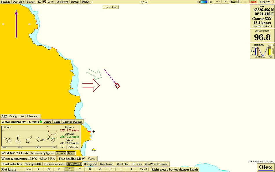
The panel displays the wind speed and direction at the moment, average wind speed for the last 10 minutes, and relative wind speed and direction. The graphs shows the wind speed over some time, and the arrows in the lower panel shows the variation in wind direction.
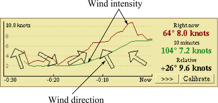
The graphs can display wind data for the past 24 hours.
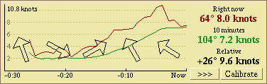
The timeline view can be changed by clicking the arrow in the lower right.
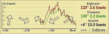
Calibrating the wind speed sensor
To get an accurate measurement of wind direction and speed, the anemometer must be placed in parallel with the vessels center line. Measure the eviation relative to the centerline, click Calibrate and enter the offset value.
Click Ok to save and exit, or click Cancel to exit without saving.
Water temperature
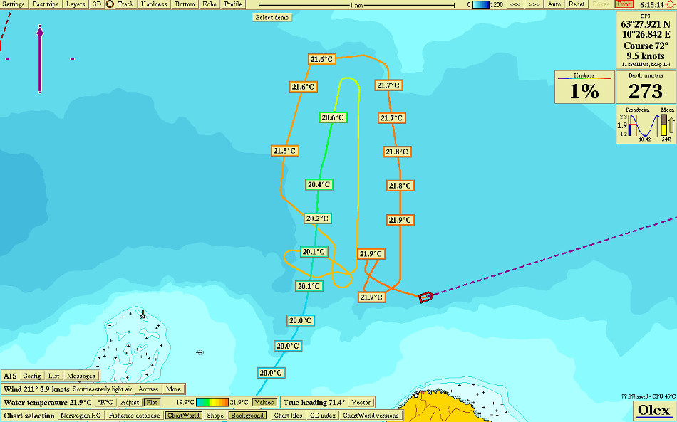
The temperature in the upper water layers can be measured either by a separate temperature sensor or an integrated temperature sensor in the echosounder. The value is displayed in the Temperature panel in the lower left part of the screen.

 - Changes the temperature unit between Fahrenheit and Celsius.
 - If the measured temperature differs from the real water temperature,
press the Adjust button to enter the offset in the text box.
- If the measured temperature differs from the real water temperature,
press the Adjust button to enter the offset in the text box.
 - By clicking Plot, the temperature panel expands and a color palette will open.
This palette shows 10 colors, evenly distributed in the interval between the minimum- and maximum temperature.
- By clicking Plot, the temperature panel expands and a color palette will open.
This palette shows 10 colors, evenly distributed in the interval between the minimum- and maximum temperature.

The lowest part of the temperature scale is shown in blue tones, and the highest part in red tones. The minimum and maximum temperatures are displayed respectively on left and right side of the color palette. Press Values to open tags showing the numerical values along the track. Hover the pointer over the tag to see the time when the temperature was measured.
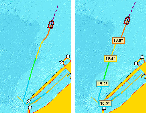
Oceanic currents
On the basis of measured positions, heading data, and water speed the Olex system can calculate the osceanic currents.
Surface current
The current is calculated continuously on the basis of recent measurements from GPS, heading sensor and the water speed sensor. The panel on the left displays the current - i.e. which way the ship is going to drift if the engine power is stopped. By clicking on Arrow, the current is visualized as an arrow pointing away from the vessel.
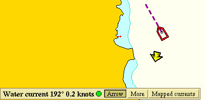
Current map
The moon's position relative to earth is considered to be the main source of tidal currents. The Olex system calculates ocean currents in relation to the �lunar half day�, having a duration equivalent to the tidal rhythm. The lunar half day is divided into 12 lunar hours, and by observing the current in the individual lunar hours, Olex can calculate future ocean currents. The ocean is divided into a grid, similar to the depth boxes, but with a slightly coarser resolution. Each square - current box, contains a set of observations related to the timing of the lunar half day. In addition to the measured currents at the moment, the measurements are stored in the current boxes and builds up a detailed map. Each set of measurements is represented by an arrow that shows the current speed and direction. Click Mapped currents to view the map.
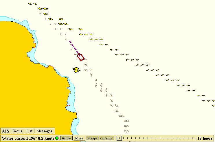
The timescale makes it possible to display a projection of currents in the next 18 hours. Drag the slider on the time scale to the right to show the estimated currents in the near future.
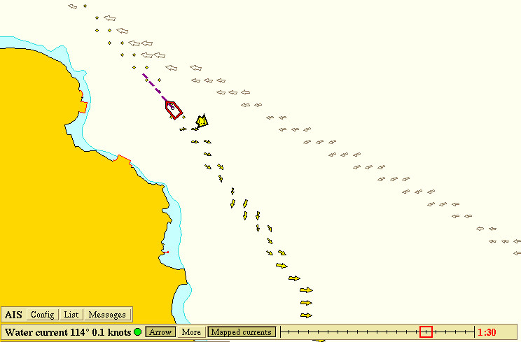
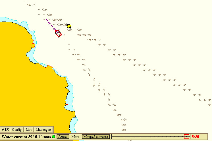
The yellow arrows in the current map shows how the computer has calculeted the currents at a particular time. The white arrows applies to other periods.

When the cursor is moved over one of the arrows, a flag opens indicating whether there are former measurements or not.
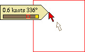
The brown field represents the lunar half day, where previous measurements are highlighted in yellow. The red marker shows the current lunar time. Clicking on More will open a list of parameters - an overview of the forces acting on the vessel at the moment.

Red values means that the parameters are outside the acceptable range, this can occur when the vessel is turning, the speed changes, or at high tides. The calulation will stop, and no values are stored.
Calibrating the wather speed sensor
The water speed sensor must be calibrated to get the best results of the measurements. Select a starting course with minimal drift and click More → Calibrate. Olex has a special mode where it asks the skipper to steer opposing straight lines at various speeds, automatically working out a graph of apparent water speed and correction factors.
- Select a starting cource with minimal lateral drift, then Start Calibration
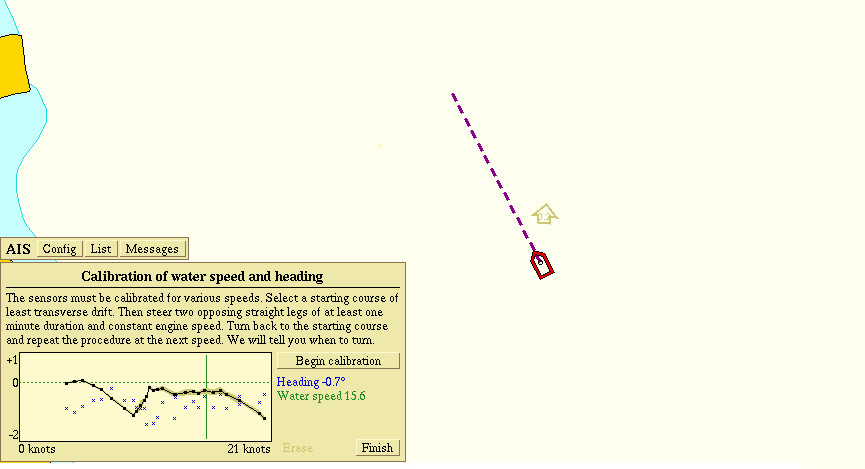
- Follow the course that the system proposes at minimum of 1 minute. Use of autopilot i srecommended.
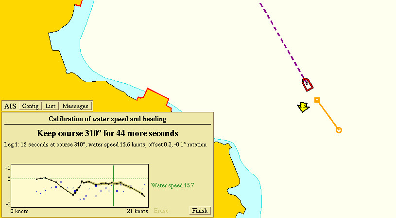
- Follow the further instructions given by the system.
- When the calibration is completed click Done.
ITI
Trawl positioning
Olex can be equipped with the trawl positioning systems Simrad ITI or Geonet IxSea. Sensors attached to the trawldoors visualizes the trawl in 2D and 3D with distance from the ship, direction, track and distance between the trawl doors. The sensors provides signals to Olex, showing the trawls location as a symbol towed behind the ship.
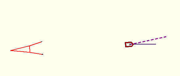
It is important to ensure that the sensors are placed correctly on the trawl. If the sensors on the starboard and port trawl door are interchanged, wrong values are used for calculating the trawls position. The sensors are shown as square boxes on the trawl symbol. Clicking on the boxes, opens a panel with information about the trawls condition. Each sensor has a panel that can be opened independently of the others.
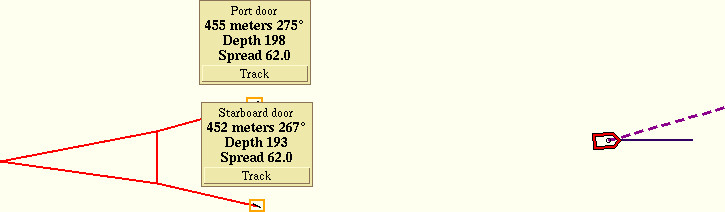
The panel shows the status of the port door with distance and direction from the ship, and the trawl depth and distance to the starboard door.
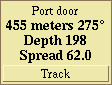
Track
Click on Track to start logging of the track for the trawl sensor. The sensors are exposed to some noise, and Olex perform a filtering of the recieved signals. Because of this, the track may have some inaccuracy in relation to the real movement.
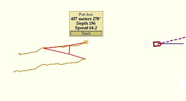
3D view
Click on 3D in the main menu to open a 3D image showing the trawl.
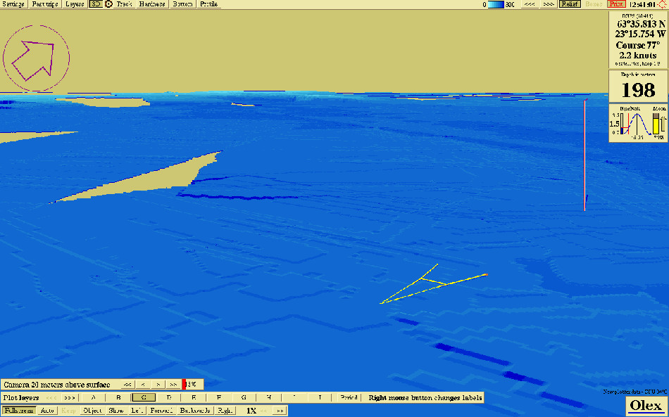
Sound Navigation and Ranging
Sonars detects an echo of their own transmitted sound signals. A directional ultrasonic pulse is emitted from a transducer, and when the pulse hits an object, the sound is reflected and captured by the transducer. From this echo the depth, speed, direction of the sonar targets extent is calculated. Olex visualizes sonar targets as small green boxes with direction, the symbols is drawn in the center of the sonar objects.

When the mouse cursor touches one of the sonar targets, text line that shows the estimated depth, area and volume of object opens. In addition, a panel opens that shows the target's assigned ID, direction and distance from own ship. Click once inside the panel to keep it open.
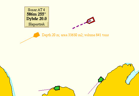
Clicking on Track to start recording the sonar targets track. The start mark is automatically labeled wiith estimated depth, area and volume of the sonar target.
Seafloor hardness
The HT-software can be used by echo sounders with BI500 interface, like Simrad the ES60 - and ES70 family. Raw data from the sonar are sent to Olex, and the system can calculate the seabed topography and hardness.The calculation is done based on the seabed�s ability to reflect sound signals, adjusted for factors that can affect the measurements. Without the HT-software, data from the Simrad echo sounder will be treated as data from a common echo sounder, where only the depth values are transferred via serial cable. The hardness is displayed in colors, each color representing a hardness value. Click Hardness in the main manu to turn on the view.

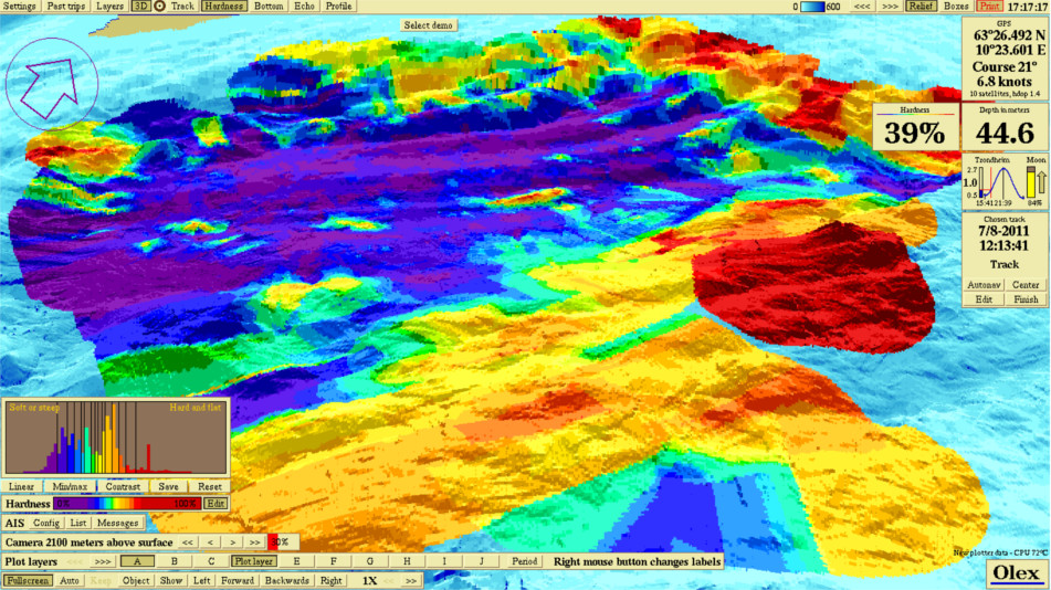
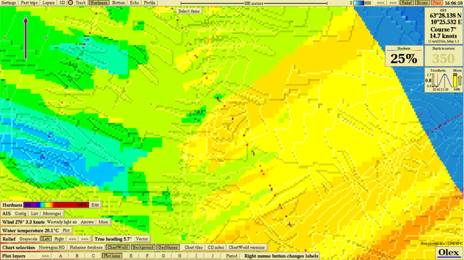
Hardness colors
The panel at the lower left shows the hardness colors spread on a scale from 0% to 100%.

Click Edit to open a view of the of hardness colors used in the visible screen.

The buttons at the bottom of the window are used to change the color spread.
 The colors are spread linearly from 0% to 100%. Each color will always have the same hardness.
 The colors are spread evenly from the lowest to the highest value.
 If an area has little variation in hardness values, the columns may have almost the same color.
Contrast spreads all hardness colors, so there will be higher contrast between the different values.
If an area has little variation in hardness values, the columns may have almost the same color.
Contrast spreads all hardness colors, so there will be higher contrast between the different values.
 Current color setting is stored as a color profile.
 Loads a previously stored color profile.
Changing the color settings, do not change the hardness values stored in the system. The colors can be adjusted, but the colors mutual location can not be changed.
Echogram
To open the traditional view of the sonar window, click on Echo in the main menu.
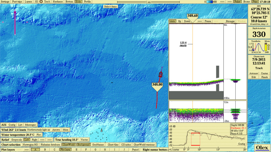
The echogram opens to the right, and a red line is displayed on the screen that shows the echograms extent.
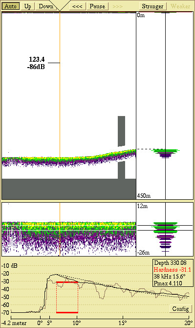
The echogram consists of 3 parts. The left part displays the water column, the right part displays a detailed view of the last sounding. The bottom echogram shows a detailed picture of the echo, without depth values.
Depth scale
The depth scale is determined by settings in the echo sounder. When the cursor is moved into the echogram ,a line appears. A flag displays the depth in that point. The corresponding depth flag is also displayed on the map. The cursor can be moved up or down to show the depth in the water column, and the attenuation of the echo.
The buttons Auto, Up and Down moves the echogram in the water column.
- Auto scales the echogram automatically.
- Up or Down moves the echogram manually.
History
The arrows at the top of the echogram window can be used to scroll back and forth in historical echogram data. Pause freezes the echogram. The end points are named with the letters A and B, the echogram thus displays the section from A to B on the map.
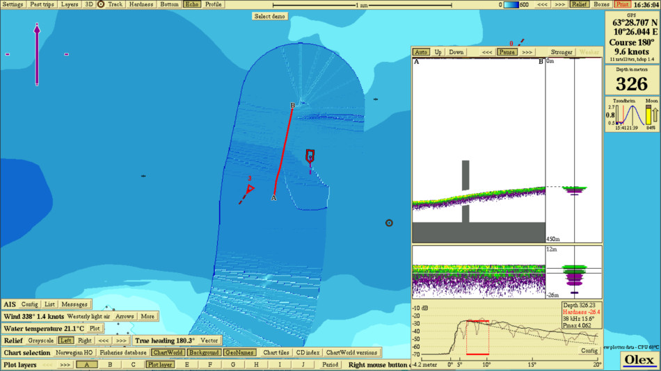
The arrows <<< and >>> moves the echogram each time you click on one of the buttons, the track moves accordingly.
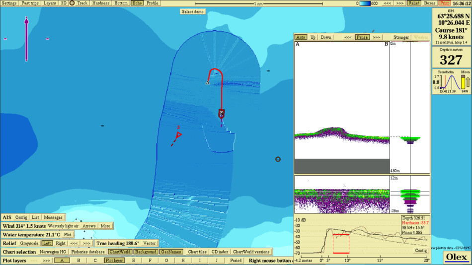
Move the mouse cursor inside the window, press and hold the schrollwheel to to move the echogram. Or press both buttons on a two-button mouse. When Pause is disabled, the echogram returns to its normal mode again.
Adjusting the signal strength
The buttons Stronger and Weaker changes the signal strength of the echo, Stronger amplifies the echo so details becomes more perceptible on the graph. The disadvantage is that the noise is amplified as well. Weaker reduces the amplification of the echo.
Details of hardness calculation
The graph shows details of the hardness calculation.
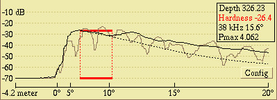
The light gray curve shows the spread of the last sounding. The dark gray curve shows the average of the last 100 soundings and the dashed line shows a theoretical average of the spread of sound. The red frame shows the area for the hardness calculation.
ARPA
ARPA targets
Olex can detect and view ARPA targets. The targets are displayed as triangle symbols, and each target is assigned to a unique ID by the radar.
 Gray icon means that the ARPA target has an uncertain position.
 Red symbol means that the ARPA target has a confirmed position.
 When one of the targets is touched by the mouse cursor a panel with information about the target's speed and course,
and the distance to own ships, opens. Click once inside the window to keep it open.
When one of the targets is touched by the mouse cursor a panel with information about the target's speed and course,
and the distance to own ships, opens. Click once inside the window to keep it open.
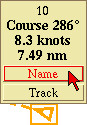 When the cursor is moved into the panel, the buttons Name and Track are added.
The panel is closed by clicking once inside the window.
When the cursor is moved into the panel, the buttons Name and Track are added.
The panel is closed by clicking once inside the window.
Click on Name and type the name in the text box that appears.

Click Ok to confirm.
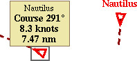
The name replaces the previous ID.
Tracks
Tracks from ARPA targets
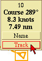 Clicking Track starts logging the ARPA targets track. The start tag gets the same name as the ARPA target.
A red frame around the symbol indicates that the track is being logged.
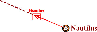
Open Layers → Default settings for new data, and select Automatic storing of radar tracks to log tracks for all ARPA targets automatically.
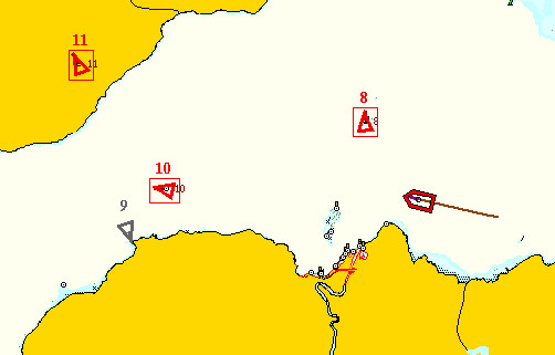
Note that to stop the logging of ARPA tracks, the logging of each target must be turned off manually. Activate Info → Present trip to display the tracks for all ARPA targets. If an ARPA target disappears, the track will also disappear.
3D view
Click on 3D in the top menu to open a 3D image showing all ARPA targets within range. The features of the 3D viewer used in the same way as usual.
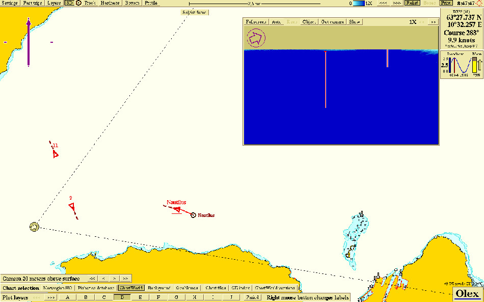
XYZ-export

Self-measured seafloor data from Olex can be exported to other 3D-modeling systems using the Export function. This data contains depth values with corresponding GPS positions and are stored as a text file in ASCII format. Plotter data such as marks and line objects are not included in the XYZ-eksport.The data are stored in a compressed file in ".gz" format. Users who need to export seafloor data can access the function by adding a DX-nokkel in Olex.
Export of seafloor data limited by a defined area
First create an area by drag and drop markers from the Main menu line.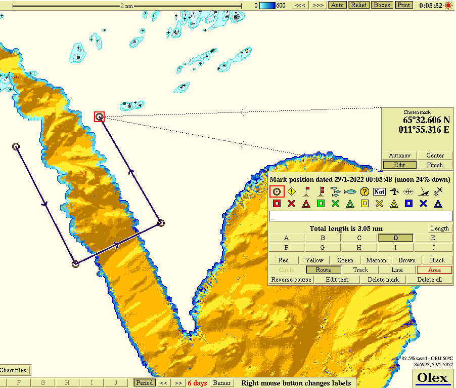
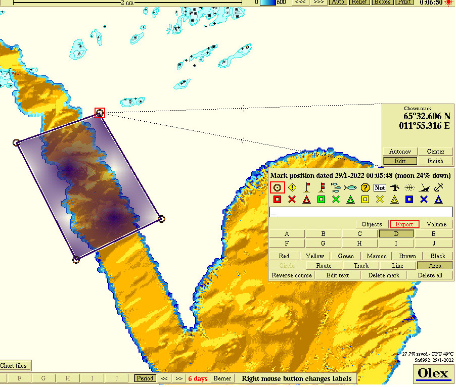
Select where to save the file and confirm, the panel will close when the export file is saved.
NMEA sentences
NMEA 0183 Sentences
| Sentence | Information | Instrument |
|---|---|---|
| ABK | Adressed and binary broadcast acknowledgement | AIS |
| CUR | Water current layer | Waterspeed sensor |
| DBS | Depth below surface | Echo sounder |
| DBT | Depth below transducer | Echo sounder |
| DPT | Depth of water | Echo sounder |
| GGA | Global positioning system fix data | GPS |
| HDG | Heading, deviation and variation | Gyro-compass, GPS-compass. satelite-compass |
| HDM | Heading magnetic | Magnet compass |
| HDT | Heading true | Gyro-compass, GPS-compass, satelite-compass |
| MTW | Water temperature | temperature sensor |
| MWD | Wind direction and speed | windspeed sensor |
| MWV | Wind speed and angle | windspeed sensor |
| OSD | Own ship data | AIS |
| RMC | Recommended minimun navigation information | GPS, autopilot |
| TTM | Tracked target message | ARPA |
| TLL | Target latitude and longitude | |
| VBW | Dual ground water speed | windspeed sensor |
| VDM | AIS and VHF data link meggages | AIS |
| VDO | AIS data link own vessel report | AIS |
| VTG | Track made good and ground speed | GPS |
| ZDA | Time and date | GPS |
From Olex to AIS and autopilot
| Sentence | Information | Instrument |
|---|---|---|
| APB | Autopilot B sentence | |
| RMB | Recommended navigation data for gps | |
| VTG | Track made good and ground speed | |
| XTE | MEasured cross track error |